6.11: Crystal Field Stabilization Energy

The difference in energy between the two sets of d orbitals is called the crystal field splitting energy (Δ_o), where the subscript o stands for octahedral. The magnitude of the splitting depends on the charge on the metal ion, the position of the metal in the periodic table, and the nature of the ligands. Crystal field splitting energy also applies to tetrahedral complexes (Δ_t), where the subscript t standands for tetrahedral. It is important to note that the splitting of the d orbitals in a crystal field does not change the total energy of the five d orbitals. In an octahedral complex, the two e_g orbitals increase in energy by 0.6Δ_o, and the three t_2g orbitals decrease in energy by 0.4Δ_o (Figure \(\PageIndex{1}\)). Thus the total change in energy is

\[ \text{CFSE}= \left[ -\frac{2}{5} \left( \text{# of electrons in } t_{2g}\right) + \frac{3}{5} \left( \text{# of electrons in } e_g \right) \right] \times \Delta_o \nonumber \]

Figure \(\PageIndex{1}\): Crystal field diagram of an octahedral complex showing the increased energy of the e_g and decreased energy of the t_2g orbitals. (LibreText)

Crystal field splitting does not change the total energy of the d orbitals.

Quantifying Crystal Field Stabilization Energy

Recall that stable molecules contain more electrons in the lower-energy (bonding) molecular orbitals in a molecular orbital diagram than in the higher-energy (antibonding) molecular orbitals. If the lower-energy set of d orbitals (the t_2g orbitals) is selectively populated by electrons, then the stability of the complex increases relative to the d-orbitals on the free metal ion. For example, the single d electron in a d¹ complex such as [Ti(H₂O)₆]³⁺ is located in one of the t_2g orbitals. Consequently, this complex will be more stable than expected on purely electrostatic grounds by 0.4Δ_o. The additional stabilization of a metal complex by selective population of the lower-energy d orbitals is called its crystal field stabilization energy (CFSE).

The CFSE of a complex can be calculated by multiplying the number of electrons in t_2g orbitals by the energy of those orbitals (−0.4Δ_o), multiplying the number of electrons in e_g orbitals by the energy of those orbitals (+0.6Δ_o), and summing the two. Using the high-spin d⁷ configuration shown in Figure \(\PageIndex{1}\) as an example:

\[\text{CFSE}=(5 \times -0.4\Delta_o)+(2 \times 0.6\Delta_o)=-0.8\Delta_o \]

CFSEs are important for two reasons. First, the existence of CFSE nicely accounts for the difference between experimentally measured values for bond energies in metal complexes and values calculated based solely on electrostatic interactions. Second, CFSE represents relatively large amounts of energy (up to several hundred kilojoules per mole), which has important chemical consequences.

Example \(\PageIndex{1}\)

What is the Crystal Field Stabilization Energy for a low spin \(d^7\) octahedral complex?

Solution

The splitting pattern and electron configuration for both isotropic and octahedral ligand fields are compared below.

\[\text{CFSE}=(6 \times -0.4\Delta_O)+(1 \times 0.6\Delta_O)=-1.8\Delta_O \]

Table \(\PageIndex{1}\) gives CFSE values for octahedral complexes with different d electron configurations. The CFSE is highest for low-spin d⁶ complexes, which accounts in part for the extraordinarily large number of Co(III) complexes known. The other low-spin configurations also have high CFSEs, as does the d³ configuration.

Table \(\PageIndex{1}\): CFSEs for Octahedral Complexes with Different Electron Configurations (in Units of Δo)

	High Spin		CFSE (Δo)	Low Spin		CFSE (Δo)
	t2g	eg		t2g	eg
d ^0			0
d ^1	↿		0.4
d ^2	↿ ↿		0.8
d ^3	↿ ↿ ↿		1.2
d ^4	↿ ↿ ↿	↿	0.6	↿⇂ ↿ ↿		1.6
d ^5	↿ ↿ ↿	↿ ↿	0.0	↿⇂ ↿⇂ ↿		2.0
d ^6	↿⇂ ↿ ↿	↿ ↿	0.4	↿⇂ ↿⇂ ↿⇂		2.4
d ^7	↿⇂ ↿⇂ ↿	↿ ↿	0.8	↿⇂ ↿⇂ ↿⇂	↿	1.8
d ^8	↿⇂ ↿⇂ ↿⇂	↿ ↿	1.2
d ^9	↿⇂ ↿⇂ ↿⇂	↿⇂ ↿	0.6
d ^10	↿⇂ ↿⇂ ↿⇂	↿⇂ ↿⇂	0.0

Octahedral d³ and d⁸ complexes and low-spin d⁶, d⁵, d⁷, and d⁴ complexes exhibit large CFSEs.

Octahedral Preference

Similar CFSE values can be constructed for non-octahedral ligand field geometries. In an octahedral complex, the two e_g orbitals decrease in energy by 0.6Δ_t, and the three t_2g orbitals increase in energy by 0.4Δ_t (Figure \(\PageIndex{2}\)). As for octahedral complexes, the total energy of the d-orbitals in a tetrahedral complex does not change; the total change in energy is

\[ \text{CFSE}= \left[ -\frac{3}{5} \left( \text{# of electrons in } t_{2g}\right) + \frac{2}{5} \left( \text{# of electrons in } e_g \right) \right] \times \Delta_t \nonumber \]

Note: \(\Delta_o\) and \(\Delta_t\) represent different units of energy. The tetrahedral crystal field is smaller in energy than the octahedral crystal field, which contributes to the tetrahedral preference for high-spin complexes (Figure \(\PageIndex{2}\)). The following conversion may be used for comparing octahedral and tetrahedral complexes that involve same ligands only:

\[\Delta_t \approx \dfrac{4}{9} \Delta_o \label{3} \]

The CFSE for a tetrahedral complex is calculated in Table \(\PageIndex{2}\). These energies can then be compared to the octahedral CFSE to calculate a thermodynamic preference (Enthalpy-wise) for a metal-ligand combination to favor the octahedral geometry. This is quantified via a Octahedral Site Preference Energy:

\[OSPE = CFSE_{(oct)} - CFSE_{(tet)} \nonumber \]

The OSPE quantifies the preference of a complex to exhibit an octahedral geometry vs. a tetrahedral geometry. Figure \(\PageIndex{3}\) compares the CFSE for tetrahedral and octahedral high-spin complexes for each d-electron configuration. From a simple inspection of Figure \(\PageIndex{3}\), the following observations can be made:

• The OSPE is small in \(d^1\), \(d^2\), \(d^5\), \(d^6\), \(d^7\) complexes and other factors influence the stability of the complexes including steric factors.
• The OSPE is large in \(d^3\) and \(d^8\) complexes which strongly favor octahedral geometries.

Figure \(\PageIndex{2}\): A comparison of octahedral and tetrahedral crystal fields. (LibreText)

Figure \(\PageIndex{1}\): Crystal Field Stabilization Energies for both octahedral fields (\(CFSE_{oct}\)) and tetrahedral fields (\(CFSE_{tet}\)). Octahedral Site Preference Energies (OSPE) are in yellow. This is for high spin complexes. (LibreText)

Table \(\PageIndex{2}\): Octahedral Site Preference Energies (OSPE)

Total d-electrons	CFSE(Octahedral)		CFSE(Tetrahedral)		OSPE (for high spin complexes)**
	High Spin	Low Spin	Configuration	Always High Spin*
d^0	0 \(\Delta_o\)	0 \(\Delta_o\)	e^0	0 \(\Delta_t\)	0 \(\Delta_o\)
d^1	-2/5 \(\Delta_o\)	-2/5 \(\Delta_o\)	e^1	-3/5 \(\Delta_t\)	-6/45 \(\Delta_o\)
d^2	-4/5 \(\Delta_o\)	-4/5 \(\Delta_o\)	e^2	-6/5 \(\Delta_t\)	-12/45 \(\Delta_o\)
d^3	-6/5 \(\Delta_o\)	-6/5 \(\Delta_o\)	e^2t2^1	-4/5 \(\Delta_t\)	-38/45 \(\Delta_o\)
d^4	-3/5 \(\Delta_o\)	-8/5 \(\Delta_o\) + P	e^2t2^2	-2/5 \(\Delta_t\)	-19/45 \(\Delta_o\)
d^5	0 \(\Delta_o\)	-10/5 \(\Delta_o\) + 2P	e^2t2^3	0 \(\Delta_t\)	0 \(\Delta_o\)
d^6	-2/5 \(\Delta_o\)	-12/5 \(\Delta_o\) + P	e^3t2^3	-3/5 \(\Delta_t\)	-6/45 \(\Delta_o\)
d^7	-4/5 \(\Delta_o\)	-9/5 \(\Delta_o\) + P	e^4t2^3	-6/5 \(\Delta_t\)	-12/45 \(\Delta_o\)
d^8	-6/5 \(\Delta_o\)	-6/5 \(\Delta_o\)	e^4t2^4	-4/5 \(\Delta_t\)	-38/45 \(\Delta_o\)
d^9	-3/5 \(\Delta_o\)	-3/5 \(\Delta_o\)	e^4t2^5	-2/5 \(\Delta_t\)	-19/45 \(\Delta_o\)
d^10	0	0	e^4t2^6	0 \(\Delta_t\)	0 \(\Delta_o\)

Example \(\PageIndex{2}\)

For each complex, predict its structure, whether it is high spin or low spin, and the number of unpaired electrons present.

1. \([Cu(NH_3)_4]^{2+}\)
2. \([Ni(CN)_4]^{2−}\)

Solution

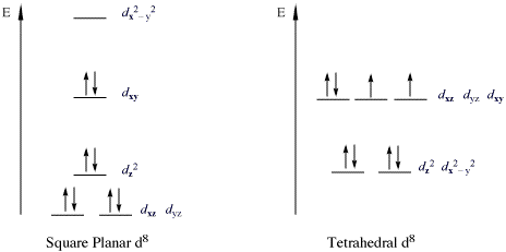
Because Δ_o is so large for the second- and third-row transition metals, all four-coordinate complexes of these metals are square planar due to the much higher crystal field stabilization energy (CFSE) for square planar versus tetrahedral structures. The only exception is for d¹⁰ metal ions such as Cd²⁺, which have zero CFSE and are therefore tetrahedral as predicted by the VSEPR model. Four-coordinate complexes of the first-row transition metals can be either square planar or tetrahedral; the former is favored by strong-field ligands, whereas the latter is favored by weak-field ligands. For example, the [Ni(CN)₄]²⁻ ion is square planar, while the [NiCl₄]²⁻ ion is tetrahedral.

1.

The copper in this complex is a d⁹ ion and it has a coordination number of 4. So it is probably either square planar or tetrahedral. To estimate which, we need to fill in the CFT splitting diagrams for each with 9 electrons and ask which has a lower energy. Comparing the square planer (Figure \(\PageIndex{1}\)) splitting diagram with tetrahedral (Figure \(\PageIndex{2}\)), suggests that 9 electrons will have a net lower total energy for square planar (since the \(d_{x^2-y^2}\) orbital is high in energy, the others are lower).

For the square planar structure, neither high nor low spin states are possible (only one state) with a single unpaired electron.

2.

The nickle in this complex is a d⁸ ion and it has a coordination number of 4. So it is probably either square planar or tetrahedral. To estimate which, we need to fill in the CFT splitting diagrams for each with 8 electrons and ask which has a lower energy. Comparing the square planer (Figure \(\PageIndex{1}\)) splitting diagram with tetrahedral (Figure \(\PageIndex{2}\)), suggests that 8 electrons will have a net lower total energy for square planar (since the \(d_{x^2-y^2}\) orbital is high in energy, the others are lower).

For the square planar structure, it is a low spin complex since a high spin requires a lot of energy to promote to the \(d_{x^2-y^2}\) orbital. Hence, there are no unpaired electrons.

Example \(\PageIndex{3}\)

Which is the preferred configuration for a d³ metal: tetrahedral or octahedral?

Solution

To answer this, the Crystal Field Stabilization Energy has to be calculated for a \((d^3\) metal in both configurations. The geometry with the greater stabilization will be the preferred geometry.

• For a d³ octahedral configuration, the Crystal Field Stabilization Energy is

\[3 \times -0.4 \Delta_o = -1.2 \Delta_o \nonumber \]

• For a d³ tetrahedral configuration (assuming high spin), the Crystal Field Stabilization Energy is

\[-0.8 \Delta_{tet} \nonumber \]

Remember that because Δ_tet is less than half the size of Δ_o, tetrahedral complexes are often high spin. We can now put this in terms of Δ_o (we can make this comparison because we're considering the same metal ion and the same ligand: all that's changing is the geometry)

So for tetrahedral d³, the Crystal Field Stabilization Energy is:

CFSE = -0.8 x 4/9 Δ_o = -0.355 Δ_o.

And the difference in Crystal Field Stabilization Energy between the two geometries will be:

1.2 - 0.355 = 0.845 Δ_o.

Example \(\PageIndex{4}\)

The molecule \(\ce{[PdCl4]^{2−}}\) is diamagnetic, which indicates a square planar geometry as all eight d-electrons are paired in the lower-energy orbitals. However, \(\ce{[NiCl4]^{2−}}\) is also d⁸ but has two unpaired electrons, indicating a tetrahedral geometry. Why is \(\ce{[PdCl4]^{2−}}\) square planar if \(\ce{Cl^{-}}\) is not a strong-field ligand?

Solution

The geometry of the complex changes going from \(\ce{[NiCl4]^{2−}}\) to \(\ce{[PdCl4]^{2−}}\). Clearly this cannot be due to any change in the ligand since it is the same in both cases. It is the other factor, the metal, that leads to the difference.

Consider the splitting of the d-orbitals in a generic d⁸ complex. If it were to adopt a square planar geometry, the electrons will be stabilized (with respect to a tetrahedral complex) as they are placed in orbitals of lower energy. However, this comes at a cost: two of the electrons, which were originally unpaired in the tetrahedral structure, are now paired in the square-planer structure:

We can label these two factors as \(ΔE\) (stabilization derived from occupation of lower-energy orbitals) and \(P\) (spin pairing energy) respectively. One can see that:

• If \(ΔE>P\), then the complex will be square planar
• If \(ΔE<P\), then the complex will be tetrahedral.

This is analogous to deciding whether an octahedral complex adopts a high- or low-spin configuration; where the crystal field splitting parameter \(Δ_o\) \(ΔE\) does above. Unfortunately, unlike \(Δ_o\) in octahedral complexes, there is no simple graphical way to represent \(ΔE\) on the diagram above since multiple orbitals are changed in energy between the two geometries.

Interpreting the origin of metal-dependent stabilization energies can be tricky. However, we know experimentally that \(\ce{Pd^{2+}}\) has a larger splitting of the d-orbitals and hence a larger \(\Delta E\) than \(\ce{Ni^{2+}}\) (moreover \(P\) is also smaller).

Practically all 4d and 5d d⁸ \(\ce{ML4}\) complexes adopt a square planar geometry, irrespective if the ligands are strong-field ligand or not. Other examples of such square planar complexes are \(\ce{[PtCl4]^{2−}}\) and \(\ce{[AuCl4]^{-}}\).

Problems

Exercise \(\PageIndex{1}\)

Determine the crystal field stabilization energy (CFSE) in the following octahedral ions:

1. \(\ce{V^3+}\)
2. \(\ce{Ni^2+}\)
3. \(\ce{Cr^3+}\)
4. \(\ce{Zn^2+}\)

Answer a

\(\ce{V^3+}\) is \(d^2\), with two electrons in the \(t_{2g}\) and zero electrons in \(e_g\).

CFSE = \([2(-0.4) + 0(0.6)]\times \Delta_o = -0.8\Delta_o\)

Answer b

\(\ce{Ni^2+}\) is \(d^8\), with six electrons in \(t_{2g}\) and two electrons in \(e_g\).

CFSE = \([6(-0.4) + 2(0.6)]\times \Delta_o = -1.2\Delta_o\)

Answer c

\(\ce{Cr^3+}\) is \(d^3\), with three electrons in \(t_{2g}\) and zero electrons in \(e_g\).

CFSE = \([3(-0.4) + 0(0.6)]\times \Delta_o = -1.2\Delta_o\)

Answer d

\(\ce{Zn^2+}\) is \(d^{10}\), with six electrons in \(t_{2g}\) and four electrons in \(e_g\).

CFSE = \([6(-0.4) + 4(0.6)]\times \Delta_o = 0\Delta_o\).

Exercise \(\PageIndex{2}\)

What are the geometries of the following two complexes?

1. \([\ce{AlCl_4}]^-\)
2. \([\ce{Ag(NH_3)_2}]^+\)

Answer 1

tetrahedral

Answer 2

linear

 

Contributors and Attributions

• Asadullah Awan (UCD), Hong Truong (UCD)

• Prof. Robert J. Lancashire (The Department of Chemistry, University of the West Indies)