5.9: Electronic Spectra of Coordination Compounds

Term Splitting for Octahedral d² metal complexes

At first glance, one might think that there is only one possible transition for the d-electrons in an octahedral compound with a d² configuration when it absorbs light. That transition would be one of the electrons in a t_2g orbital raising in energy to one of the e_g orbitals. One example of this is shown below (Figure \(\PageIndex{1}\)). This might lead you to think there is only one band (peak) in the visible absorption spectrum for d² complexes, but that is not the case. In order to explain the additional bands, there would have to be other possible transitions. Perhaps you might think that since the electrons in the t_2g orbitals are equal in energy either of them could move to the e_g. Similarly, the e_g orbitals are degenerate, so the electron could go to either of those orbitals. That could give multiple transitions, but they would all be the same energy as the one depicted.  

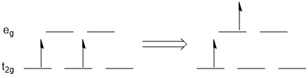
Figure \(\PageIndex{1}\). A possible transition for an electron in the t_2g orbital of a d² system.

What other transitions would be possible? The state shown above depicts the ground state electron configuration of a d² system. Remember back to general chemistry, the ground state follows Hund's rule in that the electrons are spread out and have the same spin. There are multiple possible excited states and these do not have to abide by Hund's rule, but they still must follow the Pauli exclusion principle. Several possible excited state configurations are shown below (Figure \(\PageIndex{2}\)).

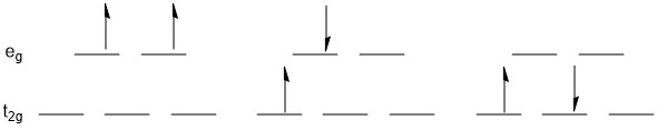
Figure \(\PageIndex{2}\). Additional possible excited states for a d² system. 

To help keep track of all of the possible transitions, we use Term Symbols. Term Symbols are a method of accounting for electron-electron interactions in an atom. They are derived from the quantum numbers, in particular the values of m_l and m_s, associated with the electrons of interest. These term symbols take the form ^2S+1L_J, where S represents the total spin angular momentum, L specifies the total orbital angular momentum, and J refers to the total angular momentum. How do we get these term symbols? The value of S comes from the sum of the m_s values for the electrons under consideration. As has typically been the case since general chemistry, the first electron we place is spin up or +\(\frac{1}{2}\). So for the ground state shown in (Figure \(\PageIndex{1}\)) the value of S would be +1. The value of 2S+1 is called the multiplicity and in this example the multiplicity would equal three. This is referred to as a triplet or triplet state.  The value of L comes from the sum of the m_l values. In the case above we are looking at d-orbitals. The possible m_l values are +2, +1, 0, -1 and -2. Standard practice is to begin filling the orbital with the highest value of m_l working to the lowest value. So for the ground state d² system, one electron would have a m_l or +2 and the other would be +1 giving a total of +3 as the value for L. However, L is not represented by this value, but rather a letter. This system is very similar to that used for the naming of atomic orbitals; an atomic orbital with an l value of 0 is an s-orbital while a term symbol with a L value of 0 would be an S term. This follows the same order as we learned for atomic orbitals, but it is very easy to get L values greater than 3, so after S, P, D, F the order proceeds G, H, K, I, etc. So far, this would make our ground state term for the d² system a ³F term. The final value in the term symbol is J (which is why the letter J was skipped in the list above). This value comes from combinations of L and S. 

The term symbols just described are known as free ion terms. This means we would be thinking about a d² metal ion in the gas phase. Things change a bit when you consider a metal with ligands. We move from the free ion terms to symbols that come from group theory. We also now have to deal with a wide range of ligands from weak field to strong field. As the ligands impact the separation of the t_2g and e_g orbitals, they should have an impact on the absorption of the complex. Doing much more with Term symbols is beyond the scope of this course. However, they do appear in the discussion below so it is important you have some appreciation of their source.

Selection Rules

In most cases the ligand field strength is in between the very weak and very strong case, and thus, we could expect very complicated spectra. Fortunately, nature does not make things quite as complicated, because not all possible electron transitions are quantum-mechanically allowed. The allowed transitions are defined by two rules: The spin selection rule and the Laporte rule.

The spin selection rule states that only transitions are allowed in which the total spin quantum number S does not change. Another way to say this is that only transitions between states with the same multiplicity are allowed. For example, it would be allowed to excite an electron from a triplet term to another triplet term, but not from a triplet term to a doublet or singlet term.

The Laporte rule state that transitions are only allowed when there is a change of parity. To fully appreciate this, we must define the terms gerade (symmetric with respect to inversion) and ungerade (not symmetric with respect to inversion). In thinking about this in terms of atomic orbitals, s-orbitals are completely spherical and as such are gerade. While it might take a little more to visualize it, d-orbitals are also gerade. On the other hand, p-orbitals, with the lobes having different signs are ungerade. This means that transitions between d-orbitals should not be allowed by the Laporte rule. However, in an octahedral geometry, it is possible that some terms may have a change in parity. So overall, a transition from a gerade (g) to an ungerade (u)-term and vice versa is possible, but not a transition from a g-term to another g-term, or the transition from a u-term to another u-term. For example the transition from a T_2g to a T_1u term would be allowed, but not the transition from a T_2g to a T_1g term.

Tanabe-Sugano diagram of a d² octahedral complex

In order to provide a somewhat quantitative way of representing the possible transitions for electrons in an octahedral compound, Tanabe-Sugano diagrams were developed (Figure \(\PageIndex{3}\)). The y-axis is energy divide by B, the Racah parameter. The Racah parameter is a quantum-mechanical energy unit for the electromagnetic interactions between the electrons. It is chosen because it provides “handy” numbers. Also on the y-axis one can find the free ion terms. The ground state is the lowest energy term. The x-axis is a measurement of the ligand field strength also given in terms of the Racah parameter. At 0, there are no ligands so we use the free ion terms. As the values on the x-axis increase so does the ligand field strength so weak-field ligands are towards the origin and strong field ligands are further away.

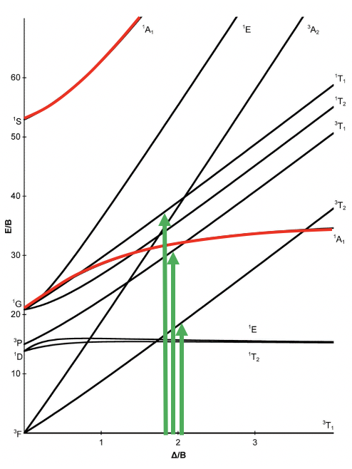
Figure \(\PageIndex{3}\). Tanabe-Sugano diagram for d² octahedral complexes. 

You can see that some lines coming from the free ion terms in the diagram are bent, and some are straight. Bending of lines occurs when two terms interact with each other because they are close in energy and have the same symmetry. This is again an analogy to orbitals. Like orbitals interact when they have the same symmetry and similar energy, terms interact when they have the same symmetry and the same energy. The closer the terms come to the point where they cross, the stronger their interactions, because their energies become more and more similar. The interactions lead to the fact that the terms bend away from each other, leading to bent curves. This means that curves for two terms of the same symmetry type will bend away in a Tanabe-Sugano diagram and never cross. For example  the terms for the two ¹A_1g terms (in red above) bend away from each other and do not cross.

Next, let us think about which electron transitions would be allowed under the consideration of the spin selection and the Laporte rule. We notice that in the symmetry labels the “g” for gerade has been omitted. This is a common simplification made in the literature but all the terms shown are “g” terms. What does this mean for the allowance of electron transitions? It suggests that no electron transition should be allowed, and that would imply that the complex could not absorb light. The Laporte selection rule however does not hold strictly. It only says that the probability of the electron-transition is reduced, however, not forbidden. This means that an absorption band that disobeys the Laporte rule will have lower intensity compared to one that follows the Laporte rule, but it still can be observed. The spin-selection rule, however, holds strictly, and transitions between terms of different spin multiplicity are strictly forbidden, meaning that they have near zero probability to occur. Overall, we can therefore excite an electron from the ³T₁ ground state to other triplet terms, namely the ³T₂, ³T₁ and the ³A₂ terms. 

Tanabe-Sugano diagram of d³ octahedral complexes

Now, let us have a look at the Tanabe-Sugano diagram for a d³ system in an octahedral ligand field (Figure \(\PageIndex{4}\)). What is the ground term? We can see the term designation on the horizontal line reads “⁴A₂”, therefore this term is the ground term. How many electron transitions from the ground state should we expect? To answer this question we need to count the number of other quartet terms. There is the ⁴T₂, the ⁴T₁, and the ⁴T₁. Thus, there are overall three electron transitions possible.

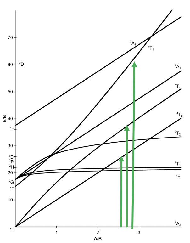
Figure \(\PageIndex{4}\). Tanabe-Sugano diagram for d³ octahedral complexes.

Tanabe-Sugano diagram of d⁴ octahedral complexes

Now let us look at the Tanabe-Sugano diagram for d⁴ octahedral complexes (Figure \(\PageIndex{5}\)). You can see that this diagram is separated into two parts separated by a vertical line. The line indicates the ligand field strength at which the complex changes from a low sping complex to a high spin complex. At lower ligand field strengths, the ground term is a ⁵E term. At higher field strength the ground term is a ³T term. For a high spin complex there is only one allowed transition because there is only one other quintet term, namely the ⁵T₂ term. For the low spin complex, there are four transitions because there are four other triplet terms.

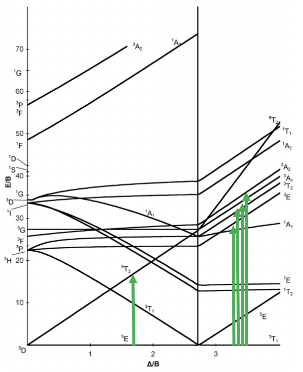
Figure \(\PageIndex{5}\). Tanabe-Sugano diagram for d⁴ octahedral complexes.

Tananbe-Sugano diagram of d⁵ octahedral complexes

The Tanabe-Sugano diagram for d⁵ octahedral complexes is divided into two parts separated by a vertical line (Figure \(\PageIndex{6}\)). The left part reflects that high spin and the right part the low spin complex. The high spin ground state is a sextet term, and the low spin ground state is a doublet term. For the high-spin complex there are no other sextet terms, meaning that there is no electron transition possible. Hence, high-spin octahedral d⁵-complexes are nearly colorless. An example for that is the hexaaqua manganese (2+) complex. A solution of this complex is near colorless, only very slightly pinkish. The slight color is because spin-forbidden transitions can occur albeit at a very low probability. For a d⁵-low spin complex there are three additional doublet states, and thus there are three electron transitions possible.

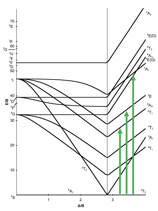
Figure \(\PageIndex{6}\). Tanabe-Sugano diagram for d⁵ octahedral complexes.

Tanabe-Sugano diagram of d⁶ octahedral complexes

The next diagram is the one for the d⁶ electron configuration (Figure \(\PageIndex{7}\)). Again, the diagram is separated into parts for high and low spin complexes. There are dotted lines in the diagram. They indicate the terms that have a different spin multiplicity than the ground term. This way we can more easily see how many electron transitions are allowed. The ground term for the high-spin complex is the quintet ⁵T₂ term. The ground term for the low spin complex is a ¹A₁ term. There is only transition allowed for the high-spin comples because the ⁵E term is the only other quintet term. There are two transitions possible for the low-spin case because there are two additional singlet terms, namely the ¹T₁ and the ¹T₂.

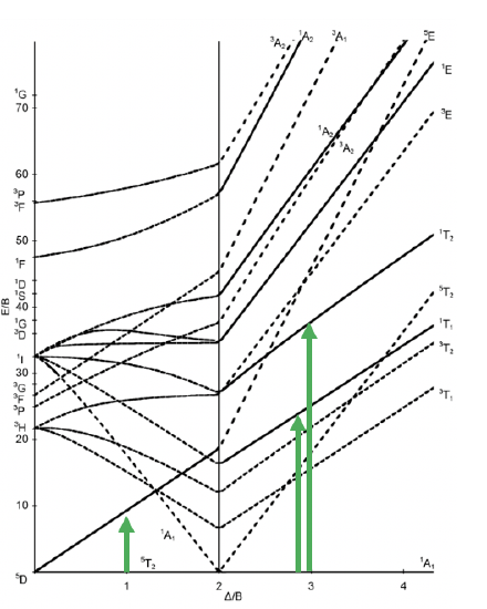
Figure \(\PageIndex{7}\). Tanabe-Sugano diagram for d⁶ octahedral complexes.

Tanabe-Sugano diagram of d⁷ octahedral complexes

Next, is the Tanabe-Sugano diagram for d⁷ octahedral complexes (Figure \(\PageIndex{8}\)). In this case, the high spin complex has a ⁴T₁ ground term, and the low spin complex has a ²E ground term. There are two other quartet terms, and two other doublet terms, hence there are two electrons transitions for the high-spin complex, and two for the low spin complex.  

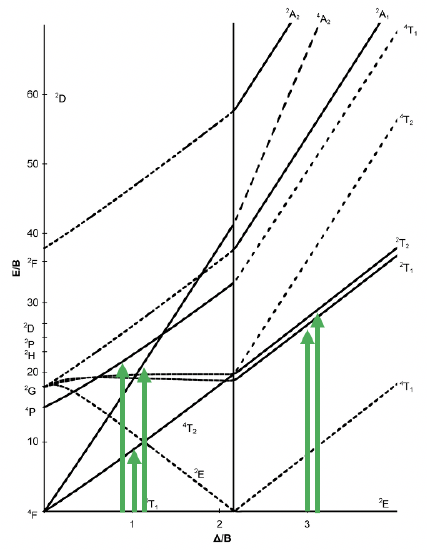
Figure \(\PageIndex{8}\). Tanabe-Sugano diagram for d⁷ octahedral complexes.

Tanabe-Sugano diagram of d⁸ octahedral complexes

Finally, we will examine the Tanabe-Sugano diagram for octahedral complexes with d⁸ electron configuration (Figure \(\PageIndex{9}\)). For this electron configuration, there are no high and low spin complexes possible, therefore, the Tanabe-Sugano diagram is no longer divided into two parts. There is a single ground term of the type ³A₂. There are three other triplet states, namely the ³T₂ and two ³T₁ terms. Therefore, there are three electron transitions possible.

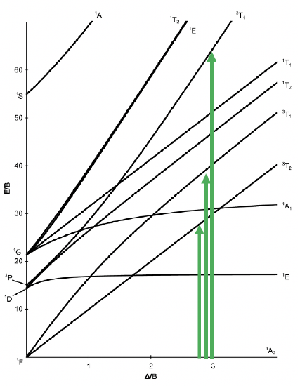
Figure \(\PageIndex{9}\). Tanabe-Sugano diagram for d⁸ octahedral complexes.

You might wonder where are the Tanabe-Sugano diagrams for d¹, d⁹, and d¹⁰? For d¹ there are no electron-electron interactions, thus a simple orbital picture is sufficient. The ²D term splits into T_2g and E_g terms, and there is only one electron transition possible. The d⁹ electron configuration is the “hole-analog” of the d¹ electron configuration. It has also just one ²D term which splits into a T_2g and an E_g term in the octahedral ligand field. Therefore, also in this case there is only one electron transition from the T_2g into the E_g term possible. In the case of d¹⁰ the orbitals are filled, and there is only the ¹S term which does not split in an octahedral ligand field. Therefore, there are no electron transitions in this case.

Finally, it should be mentioned that it is also possible to construct Tanabe-Sugano diagrams for other shapes such as the tetrahedral shape, but we will not discuss these further here.

Charge Transfer Transitions

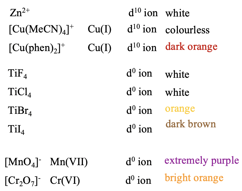
Figure 8.2.19 d-d transitions

We are still not done with our electronic spectra. Thus, far we have only considered transitions of d-electrons between d-orbitals, and their terms. They are called d-d transitions. However, there are also so-called charge transfer transitions possible, that are not d-d transitions. We can easily see that there must be other transitions but d-d transitions when we look at the color of d¹⁰ and d⁰ ions. For those, the are no d-d transitions possible. Therefore, they all should be colorless. However, that is not always true. Some of these ions are indeed colorless, but some are not. For example, Zn²⁺, a d¹⁰ ion are always colorless in complexes, but not Cu(I) which is also d¹⁰. While tetrakis(acetonitrile)copper (+) is colorless, bis(phenanthrene) copper(+) is dark orange.  Similar is true for d0 ions. While TiF₄ and TiCl₄ are colorless, TiBr₄ is orange, and TiI₄ is brown. Some d⁰ species are even extremely colorful, for example permanganate with Mn⁷⁺ which is extremely purple, and dichromate with Cr(VI) which is bright orange.

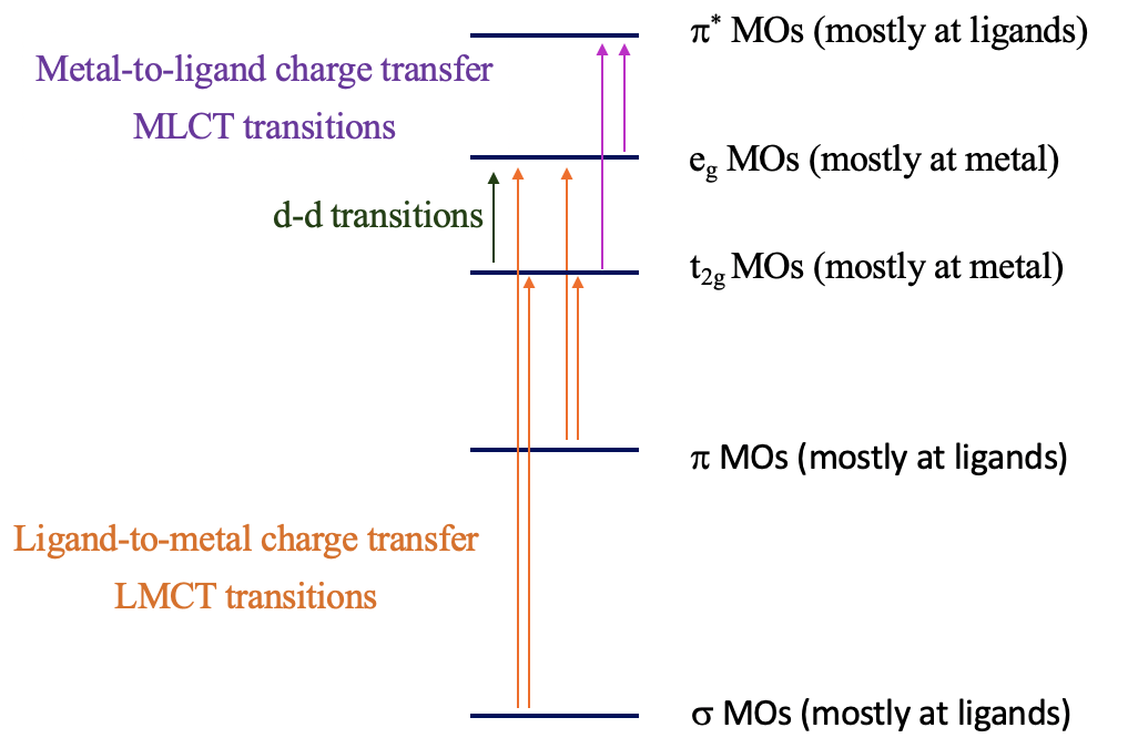
Figure 8.2.20 Charge-transfer transitions

The explanation of these phenomena are charge-transfer transitions. There are two types of charge-transfer transitions, the ligand-to-metal (LCMT) and the metal-to-ligand (MLCT) charge transfer transitions. For the ligand-to-metal transitions, electrons from bonding σ and π-orbitals get excited into metal d-orbitals in the ligand field, for example the t_2g and the e_g orbitals in an octahedral complex. If the energy difference between the σ/π-orbitals and the d-orbitals is small enough, then this electron-transition is associated with the absorption of visible light. The transition is called a ligand-to-metal transition because the ligand σ/π-orbitals are mostly located at the ligands, while the metal-d-orbitals in a ligand field are mostly located at the metal. Vice versa, the metal-to-ligand transition involves the transition of an electron from metal d-orbitals in a ligand field to ligand π*-orbitals. This essentially moves electron density from the metal to the ligand, hance the name ligand-to-metal-charge transfer transition. If the energy-difference between the ligand π* and the metal orbitals is small enough, then the absorption occurs in the visible range. Charge-transfer transitions are usually both spin- and Laporte allowed, hence if they occur the color is often very intense. How can we distinguish between d-d and charge transfer transitions? Charge transfer transitions often change in energy as the solvent polarity is varied (solvatochromic) as there is a change in polarity of the complex associated with the charge transfer transition. This can be used to distinguish between d-d transitions and charge-transfer bands.

LMCT Transitions

Can we predict when the energy windows between the bonding molecular orbitals and the metal d-orbitals are small enough so that LMCT transitions in the visible can take place?  Generally, it would be desirable if the energy of the metal orbitals was as low as possible and the energy of the bonding ligand orbitals are as high as possible. The energy of metal d-orbitals decreases with increasing positive charge at the metal because the effective nuclear charge on the metal increases. This means that very high oxidation states favor an LMCT transition. The d-orbitals should have few or no electrons, so that electrons can be promoted into the orbitals, and orbital energy increase due to electron-electron repulsion is minimized. Examples are Mn(VII), Cr(VI), and Ti(IV). The energy of MOs from bonding ligand orbitals increases when the ligand orbitals have high energy this is typically the case for π-donor ligand with negative charge.

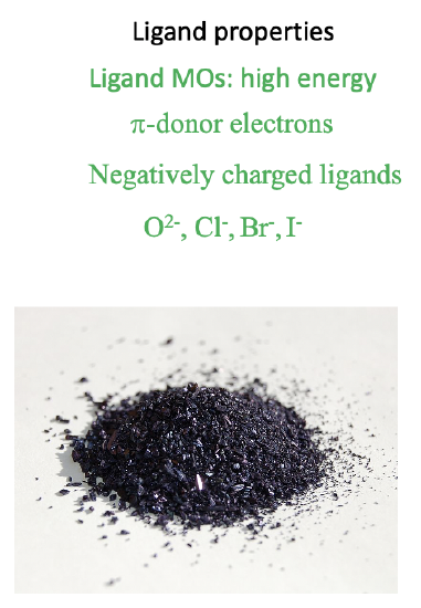
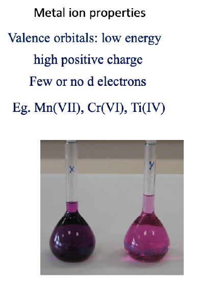
Figure 8.2.21 The properties of the metal ion and ligands in MnO₄^- (Attribution: Pradana Aumars / CC (https://commons.wikimedia.org/wiki/F...entrations.jpg))

Examples of ligands are oxo- and halo ligands. This explains for example the LMCT transitions in permanganate. The Mn is in the very high oxidation state +7, and the ligands are are oxo-ligands wich are π-donors with a 2- negative charge. The transitions are both Laporte and spin-allowed leading to very high intensity of light absorption, and thus color.

MLCT Transitions

What are favorable metal ion and ligand properties for a metal-to-ligand transition, then? In this case we would like to keep the energy of the metal orbitals as high as possible so that the energy difference between a metal d-orbital and a π*-orbital is minimized. This is accomplished when the positive charge at the metal ion is small, and there are many d-electrons that can repel each other, thereby increasing orbital energies, for examples Cu(I).

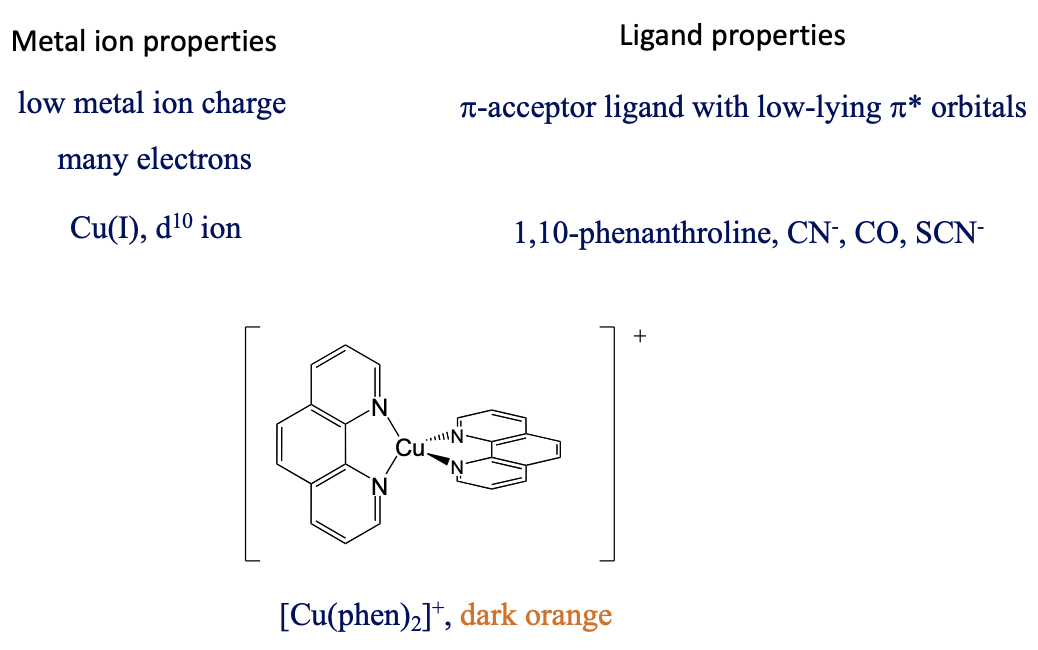
Figure 8.2.22 bis(phenanthroline) copper(+)

The ligand should be a π-acceptor with low-lying π*-orbitals, for example phenanthroline, CN^-, SCN^-, and CO. For instance, the bis(phenanthroline) copper(+) is dark-orange and has a MCLT absorption band a 458 nm. Also, the MLCT transfer is both spin and Laporte-allowed.

It should be mentioned that some complexes allow for both metal-to-ligand and ligand to metal transitions. For example, in the Cr(CO)₆ complex the σ-orbitals are high enough and the π*-orbitals are low enough in energy to allow for light absorption in the visible range. Finally, also intraligand bands are possible when the ligand is a chromophore.

---

Dr. Kai Landskron (Lehigh University). If you like this textbook, please consider to make a donation to support the author's research at Lehigh University: Click Here to Donate.

Tags recommended by the template: article:topic