
4.3: Coulometric Methods
- Page ID
- 379470

\( \newcommand{\vecs}[1]{\overset { \scriptstyle \rightharpoonup} {\mathbf{#1}} } \)
\( \newcommand{\vecd}[1]{\overset{-\!-\!\rightharpoonup}{\vphantom{a}\smash {#1}}} \)
\( \newcommand{\dsum}{\displaystyle\sum\limits} \)
\( \newcommand{\dint}{\displaystyle\int\limits} \)
\( \newcommand{\dlim}{\displaystyle\lim\limits} \)
\( \newcommand{\id}{\mathrm{id}}\) \( \newcommand{\Span}{\mathrm{span}}\)
( \newcommand{\kernel}{\mathrm{null}\,}\) \( \newcommand{\range}{\mathrm{range}\,}\)
\( \newcommand{\RealPart}{\mathrm{Re}}\) \( \newcommand{\ImaginaryPart}{\mathrm{Im}}\)
\( \newcommand{\Argument}{\mathrm{Arg}}\) \( \newcommand{\norm}[1]{\| #1 \|}\)
\( \newcommand{\inner}[2]{\langle #1, #2 \rangle}\)
\( \newcommand{\Span}{\mathrm{span}}\)
\( \newcommand{\id}{\mathrm{id}}\)
\( \newcommand{\Span}{\mathrm{span}}\)
\( \newcommand{\kernel}{\mathrm{null}\,}\)
\( \newcommand{\range}{\mathrm{range}\,}\)
\( \newcommand{\RealPart}{\mathrm{Re}}\)
\( \newcommand{\ImaginaryPart}{\mathrm{Im}}\)
\( \newcommand{\Argument}{\mathrm{Arg}}\)
\( \newcommand{\norm}[1]{\| #1 \|}\)
\( \newcommand{\inner}[2]{\langle #1, #2 \rangle}\)
\( \newcommand{\Span}{\mathrm{span}}\) \( \newcommand{\AA}{\unicode[.8,0]{x212B}}\)
\( \newcommand{\vectorA}[1]{\vec{#1}} % arrow\)
\( \newcommand{\vectorAt}[1]{\vec{\text{#1}}} % arrow\)
\( \newcommand{\vectorB}[1]{\overset { \scriptstyle \rightharpoonup} {\mathbf{#1}} } \)
\( \newcommand{\vectorC}[1]{\textbf{#1}} \)
\( \newcommand{\vectorD}[1]{\overrightarrow{#1}} \)
\( \newcommand{\vectorDt}[1]{\overrightarrow{\text{#1}}} \)
\( \newcommand{\vectE}[1]{\overset{-\!-\!\rightharpoonup}{\vphantom{a}\smash{\mathbf {#1}}}} \)
\( \newcommand{\vecs}[1]{\overset { \scriptstyle \rightharpoonup} {\mathbf{#1}} } \)
\(\newcommand{\longvect}{\overrightarrow}\)
\( \newcommand{\vecd}[1]{\overset{-\!-\!\rightharpoonup}{\vphantom{a}\smash {#1}}} \)
\(\newcommand{\avec}{\mathbf a}\) \(\newcommand{\bvec}{\mathbf b}\) \(\newcommand{\cvec}{\mathbf c}\) \(\newcommand{\dvec}{\mathbf d}\) \(\newcommand{\dtil}{\widetilde{\mathbf d}}\) \(\newcommand{\evec}{\mathbf e}\) \(\newcommand{\fvec}{\mathbf f}\) \(\newcommand{\nvec}{\mathbf n}\) \(\newcommand{\pvec}{\mathbf p}\) \(\newcommand{\qvec}{\mathbf q}\) \(\newcommand{\svec}{\mathbf s}\) \(\newcommand{\tvec}{\mathbf t}\) \(\newcommand{\uvec}{\mathbf u}\) \(\newcommand{\vvec}{\mathbf v}\) \(\newcommand{\wvec}{\mathbf w}\) \(\newcommand{\xvec}{\mathbf x}\) \(\newcommand{\yvec}{\mathbf y}\) \(\newcommand{\zvec}{\mathbf z}\) \(\newcommand{\rvec}{\mathbf r}\) \(\newcommand{\mvec}{\mathbf m}\) \(\newcommand{\zerovec}{\mathbf 0}\) \(\newcommand{\onevec}{\mathbf 1}\) \(\newcommand{\real}{\mathbb R}\) \(\newcommand{\twovec}[2]{\left[\begin{array}{r}#1 \\ #2 \end{array}\right]}\) \(\newcommand{\ctwovec}[2]{\left[\begin{array}{c}#1 \\ #2 \end{array}\right]}\) \(\newcommand{\threevec}[3]{\left[\begin{array}{r}#1 \\ #2 \\ #3 \end{array}\right]}\) \(\newcommand{\cthreevec}[3]{\left[\begin{array}{c}#1 \\ #2 \\ #3 \end{array}\right]}\) \(\newcommand{\fourvec}[4]{\left[\begin{array}{r}#1 \\ #2 \\ #3 \\ #4 \end{array}\right]}\) \(\newcommand{\cfourvec}[4]{\left[\begin{array}{c}#1 \\ #2 \\ #3 \\ #4 \end{array}\right]}\) \(\newcommand{\fivevec}[5]{\left[\begin{array}{r}#1 \\ #2 \\ #3 \\ #4 \\ #5 \\ \end{array}\right]}\) \(\newcommand{\cfivevec}[5]{\left[\begin{array}{c}#1 \\ #2 \\ #3 \\ #4 \\ #5 \\ \end{array}\right]}\) \(\newcommand{\mattwo}[4]{\left[\begin{array}{rr}#1 \amp #2 \\ #3 \amp #4 \\ \end{array}\right]}\) \(\newcommand{\laspan}[1]{\text{Span}\{#1\}}\) \(\newcommand{\bcal}{\cal B}\) \(\newcommand{\ccal}{\cal C}\) \(\newcommand{\scal}{\cal S}\) \(\newcommand{\wcal}{\cal W}\) \(\newcommand{\ecal}{\cal E}\) \(\newcommand{\coords}[2]{\left\{#1\right\}_{#2}}\) \(\newcommand{\gray}[1]{\color{gray}{#1}}\) \(\newcommand{\lgray}[1]{\color{lightgray}{#1}}\) \(\newcommand{\rank}{\operatorname{rank}}\) \(\newcommand{\row}{\text{Row}}\) \(\newcommand{\col}{\text{Col}}\) \(\renewcommand{\row}{\text{Row}}\) \(\newcommand{\nul}{\text{Nul}}\) \(\newcommand{\var}{\text{Var}}\) \(\newcommand{\corr}{\text{corr}}\) \(\newcommand{\len}[1]{\left|#1\right|}\) \(\newcommand{\bbar}{\overline{\bvec}}\) \(\newcommand{\bhat}{\widehat{\bvec}}\) \(\newcommand{\bperp}{\bvec^\perp}\) \(\newcommand{\xhat}{\widehat{\xvec}}\) \(\newcommand{\vhat}{\widehat{\vvec}}\) \(\newcommand{\uhat}{\widehat{\uvec}}\) \(\newcommand{\what}{\widehat{\wvec}}\) \(\newcommand{\Sighat}{\widehat{\Sigma}}\) \(\newcommand{\lt}{<}\) \(\newcommand{\gt}{>}\) \(\newcommand{\amp}{&}\) \(\definecolor{fillinmathshade}{gray}{0.9}\)In a potentiometric method of analysis we determine an analyte’s concentration by measuring the potential of an electrochemical cell under static conditions in which no current flows and the concentrations of species in the electrochemical cell remain fixed. Dynamic techniques, in which current passes through the electrochemical cell and concentrations change, also are important electrochemical methods of analysis. In this section we consider coulometry. Voltammetry and amperometry are covered in Chapter 11.4.
Coulometry is based on an exhaustive electrolysis of the analyte. By exhaustive we mean that the analyte is oxidized or reduced completely at the working electrode, or that it reacts completely with a reagent generated at the working electrode. There are two forms of coulometry: controlled-potential coulometry, in which we apply a constant potential to the electrochemical cell, and controlled-current coulometry, in which we pass a constant current through the electrochemical cell.
During an electrolysis, the total charge, Q, in coulombs, that passes through the electrochemical cell is proportional to the absolute amount of analyte by Faraday’s law
where n is the number of electrons per mole of analyte, F is Faraday’s constant (96 487 C mol–1), and NA is the moles of analyte. A coulomb is equivalent to an A•sec; thus, for a constant current, i, the total charge is
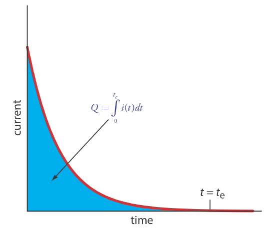
where te is the electrolysis time. If the current varies with time, as it does in controlled-potential coulometry, then the total charge is
\[Q=\int_{0}^{t_e} i(t) d t \label{11.3}\]
In coulometry, we monitor current as a function of time and use either Equation \ref{11.2} or Equation \ref{11.3} to calculate Q. Knowing the total charge, we then use Equation \ref{11.1} to determine the moles of analyte. To obtain an accurate value for NA, all the current must oxidize or reduce the analyte; that is, coulometry requires 100% current efficiency or an accurate measurement of the current efficiency using a standard.
Current efficiency is the percentage of current that actually leads to the analyte’s oxidation or reduction.
Controlled-Potential Coulometry
The easiest way to ensure 100% current efficiency is to hold the working electrode at a constant potential where the analyte is oxidized or reduced completely and where no potential interfering species are oxidized or reduced. As electrolysis progresses, the analyte’s concentration and the current decrease. The resulting current-versus-time profile for controlled-potential coulometry is shown in Figure 11.3.1 . Integrating the area under the curve (Equation \ref{11.3}) from t = 0 to t = te gives the total charge. In this section we consider the experimental parameters and instrumentation needed to develop a controlled-potential coulometric method of analysis.
Selecting a Constant Potential
To understand how an appropriate potential for the working electrode is selected, let’s develop a constant-potential coulometric method for Cu2+ based on its reduction to copper metal at a Pt working electrode.
\[\mathrm{Cu}^{2+}(a q)+2 e^{-} \rightleftharpoons \mathrm{Cu}(s) \label{11.4}\]
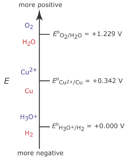
Figure 11.3.2 shows a ladder diagram for an aqueous solution of Cu2+. From the ladder diagram we know that reaction \ref{11.4} is favored when the working electrode’s potential is more negative than +0.342 V versus the standard hydrogen electrode. To ensure a 100% current efficiency, however, the potential must be sufficiently more positive than +0.000 V so that the reduction of H3O+ to H2 does not contribute significantly to the total current flowing through the electrochemical cell.
We can use the Nernst equation for reaction \ref{11.4} to estimate the minimum potential for quantitatively reducing Cu2+.
\[E=E_{\mathrm{Cu}^{2+} / \mathrm{Cu}}^{\mathrm{o}}-\frac{0.05916}{2} \log \frac{1}{\left[\mathrm{Cu}^{2+}\right]} \label{11.5}\]
So why are we using the concentration of Cu2+ in Equation \ref{11.5} instead of its activity? In potentiometry we use activity because we use Ecell to determine the analyte’s concentration. Here we use the Nernst equation to help us select an appropriate potential. Once we identify a potential, we can adjust its value as needed to ensure a quantitative reduction of Cu2+. In addition, in coulometry the analyte’s concentration is given by the total charge, not the applied potential.
If we define a quantitative electrolysis as one in which we reduce 99.99% of Cu2+ to Cu, then the concentration of Cu2+ at te is
\[\left[\mathrm{Cu}^{2+}\right]_{t_{e}}=0.0001 \times\left[\mathrm{Cu}^{2+}\right]_{0} \label{11.6}\]
where [Cu2+]0 is the initial concentration of Cu2+ in the sample. Substituting Equation \ref{11.6} into Equation \ref{11.5} allows us to calculate the desired potential.
\[E=E_{\mathrm{Cu}^{2+} / \mathrm{Cu}}^{\circ}-\frac{0.05916}{2} \log \frac{1}{0.0001 \times\left[\mathrm{Cu}^{2+}\right]} \nonumber\]
If the initial concentration of Cu2+ is \(1.00 \times 10^{-4}\) M, for example, then the working electrode’s potential must be more negative than +0.105 V to quantitatively reduce Cu2+ to Cu. Note that at this potential H3O+ is not reduced to H2, maintaining 100% current efficiency.
Many controlled-potential coulometric methods for Cu2+ use a potential that is negative relative to the standard hydrogen electrode—see, for example, Rechnitz, G. A. Controlled-Potential Analysis, Macmillan: New York, 1963, p.49. Based on the ladder diagram in Figure 11.3.2 you might expect that applying a potential <0.000 V will partially reduce H3O+ to H2, resulting in a current efficiency that is less than 100%. The reason we can use such a negative potential is that the reaction rate for the reduction of H3O+ to H2 is very slow at a Pt electrode. This results in a significant overpotential—the need to apply a potential more positive or a more negative than that predicted by thermodynamics—which shifts Eo for the H3O+/H2 redox couple to a more negative value.
Minimizing Electrolysis Time
In controlled-potential coulometry, as shown in Figure 11.3.1 , the current decreases over time. As a result, the rate of electrolysis—recall from Chapter 11.1 that current is a measure of rate—becomes slower and an exhaustive electrolysis of the analyte may require a long time. Because time is an important consideration when designing an analytical method, we need to consider the factors that affect the analysis time.
We can approximate the current’s change as a function of time in Figure 11.3.1 as an exponential decay; thus, the current at time t is
\[i_{t}=i_{0} e^{-k t} \label{11.7}\]
where i0 is the current at t = 0 and k is a rate constant that is directly proportional to the area of the working electrode and the rate of stirring, and that is inversely proportional to the volume of solution. For an exhaustive electrolysis in which we oxidize or reduce 99.99% of the analyte, the current at the end of the analysis, te, is
\[i_{t_{e}} \leq 0.0001 \times i_{0} \label{11.8}\]
Substituting Equation \ref{11.8} into Equation \ref{11.7} and solving for te gives the minimum time for an exhaustive electrolysis as
\[t_{e}=-\frac{1}{k} \times \ln (0.0001)=\frac{9.21}{k} \nonumber\]
From this equation we see that a larger value for k reduces the analysis time. For this reason we usually carry out a controlled-potential coulometric analysis in a small volume electrochemical cell, using an electrode with a large surface area, and with a high stirring rate. A quantitative electrolysis typically requires approximately 30–60 min, although shorter or longer times are possible.
Instrumentation
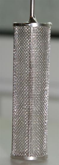
A three-electrode potentiostat is used to set the potential in controlled-potential coulometry (see Figure 11.1.5). The working electrodes is usually one of two types: a cylindrical Pt electrode manufactured from platinum-gauze (Figure 11.3.3 ), or a Hg pool electrode. The large overpotential for the reduction of H3O+ at Hg makes it the electrode of choice for an analyte that requires a negative potential. For example, a potential more negative than –1 V versus the SHE is feasible at a Hg electrode—but not at a Pt electrode—even in a very acidic solution. Because mercury is easy to oxidize, it is less useful if we need to maintain a potential that is positive with respect to the SHE. Platinum is the working electrode of choice when we need to apply a positive potential.
The auxiliary electrode, which often is a Pt wire, is separated by a salt bridge from the analytical solution. This is necessary to prevent the electrolysis products generated at the auxiliary electrode from reacting with the analyte and interfering in the analysis. A saturated calomel or Ag/AgCl electrode serves as the reference electrode.
The other essential need for controlled-potential coulometry is a means for determining the total charge. One method is to monitor the current as a function of time and determine the area under the curve, as shown in Figure 11.3.1 . Modern instruments use electronic integration to monitor charge as a function of time. The total charge at the end of the electrolysis is read directly from a digital readout.
Electrogravimetry
If the product of controlled-potential coulometry forms a deposit on the working electrode, then we can use the change in the electrode’s mass as the analytical signal. For example, if we apply a potential that reduces Cu2+ to Cu at a Pt working electrode, the difference in the electrode’s mass before and after electrolysis is a direct measurement of the amount of copper in the sample. As we learned in Chapter 8, we call an analytical technique that uses mass as a signal a gravimetric technique; thus, we call this electrogravimetry.
Controlled-Current Coulometry
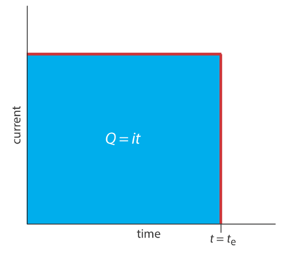
A second approach to coulometry is to use a constant current in place of a constant potential, which results in the current-versus-time profile shown in Figure 11.3.4 . Controlled-current coulometry has two advantages over controlled-potential coulometry. First, the analysis time is shorter because the current does not decrease over time. A typical analysis time for controlled-current coulometry is less than 10 min, compared to approximately 30–60 min for controlled-potential coulometry. Second, because the total charge simply is the product of current and time (Equation \ref{11.2}), there is no need to integrate the current-time curve in Figure 11.3.4 .
Using a constant current presents us with two important experimental problems. First, during electrolysis the analyte’s concentration—and, therefore, the current that results from its oxidation or reduction—decreases continuously. To maintain a constant current we must allow the potential to change until another oxidation reaction or reduction reaction occurs at the working electrode. Unless we design the system carefully, this secondary reaction results in a current efficiency that is less than 100%. The second problem is that we need a method to determine when the analyte's electrolysis is complete. As shown in Figure 11.3.1 , in a controlled-potential coulometric analysis we know that electrolysis is complete when the current reaches zero, or when it reaches a constant background or residual current. In a controlled-current coulometric analysis, however, current continues to flow even when the analyte’s electrolysis is complete. A suitable method for determining the reaction’s endpoint, te, is needed.
Maintaining Current Efficiency
To illustrate why a change in the working electrode’s potential may result in a current efficiency of less than 100%, let’s consider the coulometric analysis for Fe2+ based on its oxidation to Fe3+ at a Pt working electrode in 1 M H2SO4.
\[\mathrm{Fe}^{2+}(a q) \rightleftharpoons \text{ Fe}^{3+}(a q)+e^{-} \nonumber\]
Figure 11.3.5 shows the ladder diagram for this system. At the beginning of the analysis, the potential of the working electrode remains nearly constant at a level near its initial value.
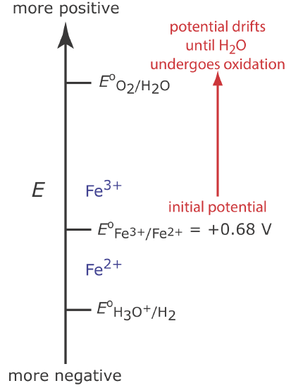
As the concentration of Fe2+ decreases and the concentration of Fe3+ increases, the working electrode’s potential shifts toward more positive values until the oxidation of H2O begins.
\[2 \mathrm{H}_{2} \mathrm{O}(l)\rightleftharpoons \text{ O}_{2}(g)+4 \mathrm{H}^{+}(a q)+4 e^{-} \nonumber\]
Because a portion of the total current comes from the oxidation of H2O, the current efficiency for the analysis is less than 100% and we cannot use Equation \ref{11.1} to determine the amount of Fe2+ in the sample.
Although we cannot prevent the potential from drifting until another species undergoes oxidation, we can maintain a 100% current efficiency if the product of that secondary oxidation reaction both rapidly and quantitatively reacts with the remaining Fe2+. To accomplish this we add an excess of Ce3+ to the analytical solution. As shown in Figure 11.3.6 , when the potential of the working electrode shifts to a more positive potential, Ce3+ begins to oxidize to Ce4+
\[\mathrm{Ce}^{3+}(a q) \rightleftharpoons \text{ Ce}^{4+}(a q)+e^{-} \label{11.9}\]
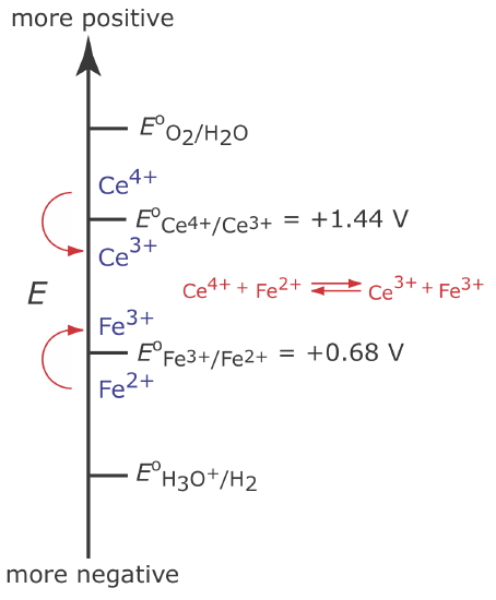
The Ce4+ that forms at the working electrode rapidly mixes with the solution where it reacts with any available Fe2+.
\[\mathrm{Ce}^{4+}(a q)+\text{ Fe}^{2+}(a q) \rightleftharpoons \text{ Ce}^{3+}(a q)+\text{ Fe}^{3+}(a q) \label{11.10}\]
Combining reaction \ref{11.9} and reaction \ref{11.10} shows that the net reaction is the oxidation of Fe2+ to Fe3+
\[\mathrm{Fe}^{2+}(a q) \rightleftharpoons \text{ Fe}^{3+}(a q)+e^{-} \nonumber\]
which maintains a current efficiency of 100%. A species used to maintain 100% current efficiency is called a mediator.
Endpoint Determination
Adding a mediator solves the problem of maintaining 100% current efficiency, but it does not solve the problem of determining when the analyte's electrolysis is complete. Using the analysis for Fe2+ in Figure 11.3.6 , when the oxidation of Fe2+ is complete current continues to flow from the oxidation of Ce3+, and, eventually, the oxidation of H2O. What we need is a signal that tells us when no more Fe2+ is present in the solution.
For our purposes, it is convenient to treat a controlled-current coulometric analysis as a reaction between the analyte, Fe2+, and the mediator, Ce3+, as shown by reaction \ref{11.10}. This reaction is identical to a redox titration; thus, we can use the end points for a redox titration—visual indicators and potentiometric or conductometric measurements—to signal the end of a controlled-current coulometric analysis. For example, ferroin provides a useful visual endpoint for the Ce3+ mediated coulometric analysis for Fe2+, changing color from red to blue when the electrolysis of Fe2+ is complete.
Reaction \ref{11.10} is the same reaction we used in Chapter 9 to develop our understanding of redox titrimetry.
Instrumentation
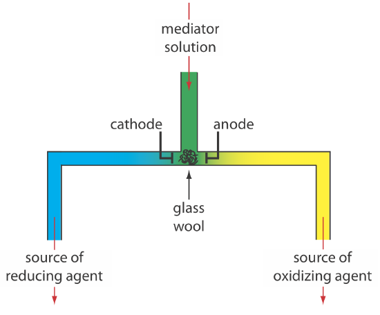
Controlled-current coulometry normally is carried out using a two-electrode galvanostat, which consists of a working electrode and a counter electrode. The working electrode—often a simple Pt electrode—also is called the generator electrode since it is where the mediator reacts to generate the species that reacts with the analyte. If necessary, the counter electrode is isolated from the analytical solution by a salt bridge or a porous frit to prevent its electrolysis products from reacting with the analyte. Alternatively, we can generate the oxidizing agent or the reducing agent externally, and allow it to flow into the analytical solution. Figure 11.3.7 shows one simple method for accomplishing this. A solution that contains the mediator flows into a small-volume electrochemical cell with the products exiting through separate tubes. Depending upon the analyte, the oxidizing agent or the reducing reagent is delivered to the analytical solution. For example, we can generate Ce4+ using an aqueous solution of Ce3+, directing the Ce4+ that forms at the anode to our sample.
Figure 11.1.4 shows an example of a manual galvanostat. Although a modern galvanostat uses very different circuitry, you can use Figure 11.1.4 and the accompanying discussion to understand how we can use the working electrode and the counter electrode to control the current. Figure 11.1.4 includes an optional reference electrode, but its presence or absence is not important if we are not interested in monitoring the working electrode’s potential.
There are two other crucial needs for controlled-current coulometry: an accurate clock for measuring the electrolysis time, te, and a switch for starting and stopping the electrolysis. An analog clock can record time to the nearest ±0.01 s, but the need to stop and start the electrolysis as we approach the endpoint may result in an overall uncertainty of ±0.1 s. A digital clock allows for a more accurate measurement of time, with an overall uncertainty of ±1 ms. The switch must control both the current and the clock so that we can make an accurate determination of the electrolysis time.
Coulometric Titrations
A controlled-current coulometric method sometimes is called a coulometric titration because of its similarity to a conventional titration. For example, in the controlled-current coulometric analysis for Fe2+ using a Ce3+ mediator, the oxidation of Fe2+ by Ce4+ (reaction \ref{11.10}) is identical to the reaction in a redox titration.
There are other similarities between controlled-current coulometry and titrimetry. If we combine Equation \ref{11.1} and Equation \ref{11.2} and solve for the moles of analyte, NA, we obtain the following equation.
\[N_{A}=\frac{i}{n F} \times t_{e} \label{11.11}\]
Compare Equation \ref{11.11} to the relationship between the moles of analyte, NA, and the moles of titrant, NT, in a titration
\[N_{A}=N_{T}=M_{T} \times V_{T} \nonumber\]
where MT and VT are the titrant’s molarity and the volume of titrant at the end point. In constant-current coulometry, the current source is equivalent to the titrant and the value of that current is analogous to the titrant’s molarity. Electrolysis time is analogous to the volume of titrant, and te is equivalent to the a titration’s end point. Finally, the switch for starting and stopping the electrolysis serves the same function as a buret’s stopcock.
For simplicity, we assumed above that the stoichiometry between the analyte and titrant is 1:1. The assumption, however, is not important and does not effect our observation of the similarity between controlled-current coulometry and a titration.
Quantitative Applications
Coulometry is used for the quantitative analysis of both inorganic and organic analytes. Examples of controlled-potential and controlled-current coulometric methods are discussed in the following two sections.
Controlled-Potential Coulometry
The majority of controlled-potential coulometric analyses involve the determination of inorganic cations and anions, including trace metals and halides ions. Table 11.3.1 summarizes several of these methods.
The ability to control selectivity by adjusting the working electrode’s potential makes controlled-potential coulometry particularly useful for the analysis of alloys. For example, we can determine the composition of an alloy that contains Ag, Bi, Cd, and Sb by dissolving the sample and placing it in a matrix of 0.2 M H2SO4 along with a Pt working electrode and a Pt counter electrode. If we apply a constant potential of +0.40 V versus the SCE, Ag(I) deposits on the electrode as Ag and the other metal ions remain in solution. When electrolysis is complete, we use the total charge to determine the amount of silver in the alloy. Next, we shift the working electrode’s potential to –0.08 V versus the SCE, depositing Bi on the working electrode. When the coulometric analysis for bismuth is complete, we determine antimony by shifting the working electrode’s potential to –0.33 V versus the SCE, depositing Sb. Finally, we determine cadmium following its electrodeposition on the working electrode at a potential of –0.80 V versus the SCE.
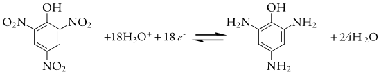
We also can use controlled-potential coulometry for the quantitative analysis of organic compounds, although the number of applications is significantly less than that for inorganic analytes. One example is the six-electron reduction of a nitro group, –NO2, to a primary amine, –NH2, at a mercury electrode. Solutions of picric acid—also known as 2,4,6-trinitrophenol, or TNP, a close relative of TNT—is analyzed by reducing it to triaminophenol.
Another example is the successive reduction of trichloroacetate to dichloroacetate, and of dichloroacetate to monochloroacetate
\[\text{Cl}_3\text{CCOO}^-(aq) + \text{H}_3\text{O}^+(aq) + 2 e^- \rightleftharpoons \text{Cl}_2\text{HCCOO}^-(aq) + \text{Cl}^-(aq) + \text{H}_2\text{O}(l) \nonumber\]
\[\text{Cl}_2\text{HCCOO}^-(aq) + \text{ H}_3\text{O}^+(aq) + 2 e^- \rightleftharpoons \text{ ClH}_2\text{CCOO}^-(aq) + \text{ Cl}^-(aq) + \text{H}_2\text{O}(l) \nonumber\]
We can analyze a mixture of trichloroacetate and dichloroacetate by selecting an initial potential where only the more easily reduced trichloroacetate reacts. When its electrolysis is complete, we can reduce dichloroacetate by adjusting the potential to a more negative potential. The total charge for the first electrolysis gives the amount of trichloroacetate, and the difference in total charge between the first electrolysis and the second electrolysis gives the amount of dichloroacetate.
Controlled-Current Coulometry (Coulometric Titrations)
The use of a mediator makes a coulometric titration a more versatile analytical technique than controlled-potential coulometry. For example, the direct oxidation or reduction of a protein at a working electrode is difficult if the protein’s active redox site lies deep within its structure. A coulometric titration of the protein is possible, however, if we use the oxidation or reduction of a mediator to produce a solution species that reacts with the protein. Table 11.3.2 summarizes several controlled-current coulometric methods based on a redox reaction using a mediator.
For an analyte that is not easy to oxidize or reduce, we can complete a coulometric titration by coupling a mediator’s oxidation or reduction to an acid–base, precipitation, or complexation reaction that involves the analyte. For example, if we use H2O as a mediator, we can generate H3O+at the anode
\[6 \mathrm{H}_{2} \mathrm{O}(l) \rightleftharpoons 4 \mathrm{H}_{3} \text{O}^{+}(a q)+\text{ O}_{2}(g)+4 e^{-} \nonumber\]
and generate OH– at the cathode.
\[2 \mathrm{H}_{2} \mathrm{O}(l)+2 e^{-} \rightleftharpoons 2 \mathrm{OH}^{-}(a q)+\text{ H}_{2}(g) \nonumber\]
If we carry out the oxidation or reduction of H2O using the generator cell in Figure 11.3.7 , then we can selectively dispense H3O+ or OH– into a solution that contains the analyte. The resulting reaction is identical to that in an acid–base titration. Coulometric acid–base titrations have been used for the analysis of strong and weak acids and bases, in both aqueous and non-aqueous matrices. Table 11.3.3 summarizes several examples of coulometric titrations that involve acid–base, complexation, and precipitation reactions.
In comparison to a conventional titration, a coulometric titration has two important advantages. The first advantage is that electrochemically generating a titrant allows us to use a reagent that is unstable. Although we cannot prepare and store a solution of a highly reactive reagent, such as Ag2+ or Mn3+, we can generate them electrochemically and use them in a coulometric titration. Second, because it is relatively easy to measure a small quantity of charge, we can use a coulometric titration to determine an analyte whose concentration is too small for a conventional titration.
Quantitative Calculations
The absolute amount of analyte in a coulometric analysis is determined using Faraday’s law (Equation \ref{11.1}) and the total charge given by Equation \ref{11.2} or by Equation \ref{11.3}. The following example shows the calculations for a typical coulometric analysis.
To determine the purity of a sample of Na2S2O3, a sample is titrated coulometrically using I– as a mediator and \(\text{I}_3^-\) as the titrant. A sample weighing 0.1342 g is transferred to a 100-mL volumetric flask and diluted to volume with distilled water. A 10.00-mL portion is transferred to an electrochemical cell along with 25 mL of 1 M KI, 75 mL of a pH 7.0 phosphate buffer, and several drops of a starch indicator solution. Electrolysis at a constant current of 36.45 mA requires 221.8 s to reach the starch indicator endpoint. Determine the sample’s purity.
Solution
As shown in Table 11.3.2 , the coulometric titration of \(\text{S}_2 \text{O}_3^{2-}\) with \(\text{I}_3^-\) is
\[2 \mathrm{S}_{2} \mathrm{O}_{3}^{2-}(a q)+\text{ I}_{3}^{-}(a q)\rightleftharpoons \text{ S}_{4} \mathrm{O}_{6}^{2-}(a q)+3 \mathrm{I}^{-}(a q) \nonumber\]
The oxidation of \(\text{S}_2 \text{O}_3^{2-}\) to \(\text{S}_4 \text{O}_6^{2-}\) requires one electron per \(\text{S}_2 \text{O}_3^{2-}\) (n = 1). Combining Equation \ref{11.1} and Equation \ref{11.2}, and solving for the moles and grams of Na2S2O3 gives
\[N_{A} =\frac{i t_{e}}{n F}=\frac{(0.03645 \text{ A})(221.8 \text{ s})}{\left(\frac{1 \text{ mol } e^{-}}{\text{mol Na}_{2} \mathrm{S}_{2} \mathrm{O}_{3}}\right)\left(\frac{96487 \text{ C}}{\text{mol } e^{-}}\right)} =8.379 \times 10^{-5} \text{ mol Na}_{2} \mathrm{S}_{2} \mathrm{O}_{3} \nonumber\]
This is the amount of Na2S2O3 in a 10.00-mL portion of a 100-mL sample; thus, there are 0.1325 grams of Na2S2O3 in the original sample. The sample’s purity, therefore, is
\[\frac{0.1325 \text{ g} \text{ Na}_{2} \mathrm{S}_{2} \mathrm{O}_{3}}{0.1342 \text{ g} \text { sample }} \times 100=98.73 \% \text{ w} / \text{w } \mathrm{Na}_{2} \mathrm{S}_{2} \mathrm{O}_{3} \nonumber\]
Note that for Equation \ref{11.1} and Equation \ref{11.2} it does not matter whether \(\text{S}_2 \text{O}_3^{2-}\) is oxidized at the working electrode or is oxidized by \(\text{I}_3^-\).
To analyze a brass alloy, a 0.442-g sample is dissolved in acid and diluted to volume in a 500-mL volumetric flask. Electrolysis of a 10.00-mL sample at –0.3 V versus a SCE reduces Cu2+ to Cu, requiring a total charge of 16.11 C. Adjusting the potential to –0.6 V versus a SCE and completing the electrolysis requires 0.442 C to reduce Pb2+ to Pb. Report the %w/w Cu and Pb in the alloy.
- Answer
-
The reduction of Cu2+ to Cu requires two electrons per mole of Cu (n = 2). Using Equation \ref{11.1}, we calculate the moles and the grams of Cu in the portion of sample being analyzed.
\[N_{C u}=\frac{Q}{n F}=\frac{16.11 \text{ C}}{\frac{2 \text{ mol } e^{-}}{\mathrm{mol} \text{ Cu}} \times \frac{96487 \text{ C}}{\text{ mol } e^{-}}}=8.348 \times 10^{-5} \text{ mol Cu} \nonumber\]
\[8.348 \times 10^{-5} \text{ mol Cu} \times \frac{63.55 \text{ g Cu} }{\text{mol Cu}}=5.301 \times 10^{-3} \text{ g Cu} \nonumber\]
This is the Cu from a 10.00 mL portion of a 500.0 mL sample; thus, the %/w/w copper in the original sample of brass is
\[\frac{5.301 \times 10^{-3} \text{ g Cu} \times \frac{500.0 \text{ mL}}{10.00 \text{ mL}}}{0.442 \text{ g sample} } \times 100=60.0 \% \text{ w/w Cu} \nonumber\]
For lead, we follow the same process; thus
\[N_{\mathrm{Pb}}=\frac{Q}{n F}=\frac{0.422 \text{ C}}{\frac{2 \text{ mol } e^-}{\text{mol Pb}} \times \frac{96487 \text{ C}}{\text{mol } e^{-}}}=2.19 \times 10^{-6} \text{ mol Pb} \nonumber\]
\[2.19 \times 10^{-6} \text{ mol Pb}\times \frac{207.2 \text{ g Pb} }{\text{mol Cu} }=4.53 \times 10^{-4} \text{ g Pb} \nonumber\]
\[\frac{4.53 \times 10^{-4} \text{ g Pb} \times \frac{500.0 \text{ mL}}{10.00 \text{ mL}}}{0.442 \text{ g sample}} \times 100=5.12 \% \text{ w/w Pb} \nonumber\]
Representative Method 11.3.1: Determination of Dichromate by a Coulometric Redox Titration
The best way to appreciate the theoretical and the practical details discussed in this section is to carefully examine a typical analytical method. Although each method is unique, the following description of the determination of \(\text{Cr}_2 \text{O}_7^{2-}\) provides an instructive example of a typical procedure. The description here is based on Bassett, J.; Denney, R. C.; Jeffery, G. H.; Mendham, J. Vogel’s Textbook of Quantitative Inorganic Analysis, Longman: London, 1978, p. 559–560.
Description of the Method
Thee concentration of \(\text{Cr}_2 \text{O}_7^{2-}\) in a sample is determined by a coulometric redox titration using Fe3+ as a mediator and electrogenerated Fe3+ as the titrant. The endpoint of the titration is determined potentiometrically.
Procedure
The electrochemical cell consists of a Pt working electrode and a Pt counter electrode placed in separate cells connected by a porous glass disk. Fill the counter electrode’s cell with 0.2 M Na2SO4, keeping the level above that of the solution in the working electrode’s cell. Connect a platinum electrode and a tungsten electrode to a potentiometer so that you can measure the working electrode’s potential during the analysis. Prepare a mediator solution of approximately 0.3 M NH4Fe(SO4)2. Add 5.00 mL of sample, 2 mL of 9 M H2SO4, and 10–25 mL of the mediator solution to the working electrode’s cell, and add distilled water as needed to cover the electrodes. Bubble pure N2 through the solution for 15 min to remove any O2 that is present. Maintain the flow of N2 during the electrolysis, turning if off momentarily when measuring the potential. Stir the solution using a magnetic stir bar. Adjust the current to 15–50 mA and begin the titration. Periodically stop the titration and measure the potential. Construct a titration curve of potential versus time and determine the time needed to reach the equivalence point.
Questions
1. Is the platinum working electrode the cathode or the anode?
Reduction of Fe3+ to Fe2+ occurs at the working electrode, making it the cathode in this electrochemical cell.
2. Why is it necessary to remove dissolved oxygen by bubbling N2 through the solution?
Any dissolved O2 will oxidize Fe2+ back to Fe3+, as shown by the following reaction.
\[4\text{Fe}^{2+}(aq) + \text{ O}_2 + \text{ 4H}_3\text{O}^+(aq) \rightleftharpoons 4\text{Fe}^{3+}(aq) + 6\text{H}_2\text{O}(l) \nonumber\]
To maintain current efficiency, all the Fe2+ must react with \(\text{Cr}_2 \text{O}_7^{2-}\). The reaction of Fe2+ with O2 means that more of the Fe3+ mediator is needed, increasing the time to reach the titration’s endpoint. As a result, we report the presence of too much \(\text{Cr}_2 \text{O}_7^{2-}\).
3. What is the effect on the analysis if the NH4Fe(SO4)2 is contaminated with trace amounts of Fe2+? How can you compensate for this source of Fe2+?
There are two sources of Fe2+: that generated from the mediator and that present as an impurity. Because the total amount of Fe2+ that reacts with \(\text{Cr}_2 \text{O}_7^{2-}\) remains unchanged, less Fe2+ is needed from the mediator. This decreases the time needed to reach the titration’s end point. Because the apparent current efficiency is greater than 100%, the reported concentration of \(\text{Cr}_2 \text{O}_7^{2-}\) is too small. We can remove trace amount of Fe2+ from the mediator’s solution by adding H2O2 and heating at 50–70oC until the evolution of O2 ceases, converting the Fe2+ to Fe3+. Alternatively, we can complete a blank titration to correct for any impurities of Fe2+ in the mediator.
4. Why is the level of solution in the counter electrode’s cell maintained above the solution level in the working electrode’s cell?
This prevents the solution that contains the analyte from entering the counter electrode’s cell. The oxidation of H2O at the counter electrode produces O2, which can react with the Fe2+ generated at the working electrode or the Cr3+ resulting from the reaction of Fe2+ and \(\text{Cr}_2 \text{O}_7^{2-}\). In either case, the result is a positive determinate error.
Characterization Applications
One useful application of coulometry is determining the number of electrons involved in a redox reaction. To make the determination, we complete a controlled-potential coulometric analysis using a known amount of a pure compound. The total charge at the end of the electrolysis is used to determine the value of n using Faraday’s law (Equation \ref{11.1}).
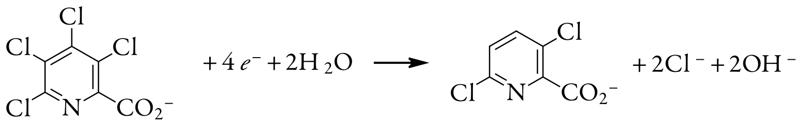
A 0.3619-g sample of tetrachloropicolinic acid, C6HNO2Cl4, is dissolved in distilled water, transferred to a 1000-mL volumetric flask, and diluted to volume. An exhaustive controlled-potential electrolysis of a 10.00-mL portion of this solution at a spongy silver cathode requires 5.374 C of charge. What is the value of n for this reduction reaction?
Solution
The 10.00-mL portion of sample contains 3.619 mg, or \(1.39 \times 10^{-5}\) mol of tetrachloropicolinic acid. Solving Equation \ref{11.1} for n and making appropriate substitutions gives
\[n=\frac{Q}{F N_{A}}=\frac{5.374 \text{ C}}{\left(96478 \text{ C/mol } e^{-}\right)\left(1.39 \times 10^{-5} \text{ mol } \mathrm{C}_{6} \mathrm{HNO}_{2} \mathrm{Cl}_{4}\right)} = 4.01 \text{ mol e}^-/\text{mol } \mathrm{C}_{6} \mathrm{HNO}_{2} \mathrm{Cl}_{4} \nonumber\]
Thus, reducing a molecule of tetrachloropicolinic acid requires four electrons. The overall reaction, which results in the selective formation of 3,6-dichloropicolinic acid, is
Evaluation
Scale of Operation
A coulometric method of analysis can analyze a small absolute amount of an analyte. In controlled-current coulometry, for example, the moles of analyte consumed during an exhaustive electrolysis is given by Equation \ref{11.11}. An electrolysis using a constant current of 100 μA for 100 s, for example, consumes only \(1 \times 10^{-7}\) mol of analyte if n = 1. For an analyte with a molecular weight of 100 g/mol, \(1 \times 10^{-7}\) mol of analyte corresponds to only 10 μg. The concentration of analyte in the electrochemical cell, however, must be sufficient to allow an accurate determination of the endpoint. When using a visual end point, the smallest concentration of analyte that can be determined by a coulometric titration is approximately 10–4 M. As is the case for a conventional titration, a coulometric titration using a visual end point is limited to major and minor analytes. A coulometric titration to a preset potentiometric endpoint is feasible even if the analyte’s concentration is as small as 10–7 M, extending the analysis to trace analytes [Curran, D. J. “Constant-Current Coulometry,” in Kissinger, P. T.; Heineman, W. R., eds., Laboratory Techniques in Electroanalytical Chemistry, Marcel Dekker Inc.: New York, 1984, pp. 539–568].
Accuracy
In controlled-current coulometry, accuracy is determined by the accuracy with which we can measure current and time, and by the accuracy with which we can identify the end point. The maximum measurement errors for current and time are about ±0.01% and ±0.1%, respectively. The maximum end point error for a coulometric titration is at least as good as that for a conventional titration, and is often better when using small quantities of reagents. Together, these measurement errors suggest that an accuracy of 0.1%–0.3% is feasible. The limiting factor in many analyses, therefore, is current efficiency. A current efficiency of more than 99.5% is fairly routine, and it often exceeds 99.9%.
In controlled-potential coulometry, accuracy is determined by current efficiency and by the determination of charge. If the sample is free of interferents that are easier to oxidize or reduce than the analyte, a current efficiency of greater than 99.9% is routine. When an interferent is present, it can often be eliminated by applying a potential where the exhaustive electrolysis of the interferents is possible without the simultaneous electrolysis of the analyte. Once the interferent is removed the potential is switched to a level where electrolysis of the analyte is feasible. The limiting factor in the accuracy of many controlled-potential coulometric methods of analysis is the determination of charge. With electronic integrators the total charge is determined with an accuracy of better than 0.5%.
If we cannot obtain an acceptable current efficiency, an electrogravimetric analysis is possible if the analyte—and only the analyte—forms a solid deposit on the working electrode. In this case the working electrode is weighed before beginning the electrolysis and reweighed when the electrolysis is complete. The difference in the electrode’s weight gives the analyte’s mass.
Precision
Precision is determined by the uncertainties in measuring current, time, and the endpoint in controlled-current coulometry or the charge in controlled-potential coulometry. Precisions of ±0.1–0.3% are obtained routinely in coulometric titrations, and precisions of ±0.5% are typical for controlled-potential coulometry.
Sensitivity
For a coulometric method of analysis, the calibration sensitivity is equivalent to nF in Equation \ref{11.1}. In general, a coulometric method is more sensitive if the analyte’s oxidation or reduction involves a larger value of n.
Selectivity
Selectivity in controlled-potential and controlled-current coulometry is improved by adjusting solution conditions and by selecting the electrolysis potential. In controlled-potential coulometry, the potential is fixed by the potentiostat, and in controlled-current coulometry the potential is determined by the redox reaction with the mediator. In either case, the ability to control the electrolysis potential affords some measure of selectivity. By adjusting pH or by adding a complexing agent, it is possible to shift the potential at which an analyte or interferent undergoes oxidation or reduction. For example, the standard-state reduction potential for Zn2+ is –0.762 V versus the SHE. If we add a solution of NH3, forming \(\text{Zn(NH}_3\text{)}_4^{2+}\), the standard state potential shifts to –1.04 V. This provides an additional means for controlling selectivity when an analyte and an interferent undergo electrolysis at similar potentials.
Time, Cost, and Equipment
Controlled-potential coulometry is a relatively time consuming analysis, with a typical analysis requiring 30–60 min. Coulometric titrations, on the other hand, require only a few minutes, and are easy to adapt to an automated analysis. Commercial instrumentation for both controlled-potential and controlled-current coulometry is available, and is relatively inexpensive. Low cost potentiostats and constant-current sources are available for approximately $1000.