9.4: Redox Titrations
- Page ID
- 165348

\( \newcommand{\vecs}[1]{\overset { \scriptstyle \rightharpoonup} {\mathbf{#1}} } \)
\( \newcommand{\vecd}[1]{\overset{-\!-\!\rightharpoonup}{\vphantom{a}\smash {#1}}} \)
\( \newcommand{\dsum}{\displaystyle\sum\limits} \)
\( \newcommand{\dint}{\displaystyle\int\limits} \)
\( \newcommand{\dlim}{\displaystyle\lim\limits} \)
\( \newcommand{\id}{\mathrm{id}}\) \( \newcommand{\Span}{\mathrm{span}}\)
( \newcommand{\kernel}{\mathrm{null}\,}\) \( \newcommand{\range}{\mathrm{range}\,}\)
\( \newcommand{\RealPart}{\mathrm{Re}}\) \( \newcommand{\ImaginaryPart}{\mathrm{Im}}\)
\( \newcommand{\Argument}{\mathrm{Arg}}\) \( \newcommand{\norm}[1]{\| #1 \|}\)
\( \newcommand{\inner}[2]{\langle #1, #2 \rangle}\)
\( \newcommand{\Span}{\mathrm{span}}\)
\( \newcommand{\id}{\mathrm{id}}\)
\( \newcommand{\Span}{\mathrm{span}}\)
\( \newcommand{\kernel}{\mathrm{null}\,}\)
\( \newcommand{\range}{\mathrm{range}\,}\)
\( \newcommand{\RealPart}{\mathrm{Re}}\)
\( \newcommand{\ImaginaryPart}{\mathrm{Im}}\)
\( \newcommand{\Argument}{\mathrm{Arg}}\)
\( \newcommand{\norm}[1]{\| #1 \|}\)
\( \newcommand{\inner}[2]{\langle #1, #2 \rangle}\)
\( \newcommand{\Span}{\mathrm{span}}\) \( \newcommand{\AA}{\unicode[.8,0]{x212B}}\)
\( \newcommand{\vectorA}[1]{\vec{#1}} % arrow\)
\( \newcommand{\vectorAt}[1]{\vec{\text{#1}}} % arrow\)
\( \newcommand{\vectorB}[1]{\overset { \scriptstyle \rightharpoonup} {\mathbf{#1}} } \)
\( \newcommand{\vectorC}[1]{\textbf{#1}} \)
\( \newcommand{\vectorD}[1]{\overrightarrow{#1}} \)
\( \newcommand{\vectorDt}[1]{\overrightarrow{\text{#1}}} \)
\( \newcommand{\vectE}[1]{\overset{-\!-\!\rightharpoonup}{\vphantom{a}\smash{\mathbf {#1}}}} \)
\( \newcommand{\vecs}[1]{\overset { \scriptstyle \rightharpoonup} {\mathbf{#1}} } \)
\(\newcommand{\longvect}{\overrightarrow}\)
\( \newcommand{\vecd}[1]{\overset{-\!-\!\rightharpoonup}{\vphantom{a}\smash {#1}}} \)
\(\newcommand{\avec}{\mathbf a}\) \(\newcommand{\bvec}{\mathbf b}\) \(\newcommand{\cvec}{\mathbf c}\) \(\newcommand{\dvec}{\mathbf d}\) \(\newcommand{\dtil}{\widetilde{\mathbf d}}\) \(\newcommand{\evec}{\mathbf e}\) \(\newcommand{\fvec}{\mathbf f}\) \(\newcommand{\nvec}{\mathbf n}\) \(\newcommand{\pvec}{\mathbf p}\) \(\newcommand{\qvec}{\mathbf q}\) \(\newcommand{\svec}{\mathbf s}\) \(\newcommand{\tvec}{\mathbf t}\) \(\newcommand{\uvec}{\mathbf u}\) \(\newcommand{\vvec}{\mathbf v}\) \(\newcommand{\wvec}{\mathbf w}\) \(\newcommand{\xvec}{\mathbf x}\) \(\newcommand{\yvec}{\mathbf y}\) \(\newcommand{\zvec}{\mathbf z}\) \(\newcommand{\rvec}{\mathbf r}\) \(\newcommand{\mvec}{\mathbf m}\) \(\newcommand{\zerovec}{\mathbf 0}\) \(\newcommand{\onevec}{\mathbf 1}\) \(\newcommand{\real}{\mathbb R}\) \(\newcommand{\twovec}[2]{\left[\begin{array}{r}#1 \\ #2 \end{array}\right]}\) \(\newcommand{\ctwovec}[2]{\left[\begin{array}{c}#1 \\ #2 \end{array}\right]}\) \(\newcommand{\threevec}[3]{\left[\begin{array}{r}#1 \\ #2 \\ #3 \end{array}\right]}\) \(\newcommand{\cthreevec}[3]{\left[\begin{array}{c}#1 \\ #2 \\ #3 \end{array}\right]}\) \(\newcommand{\fourvec}[4]{\left[\begin{array}{r}#1 \\ #2 \\ #3 \\ #4 \end{array}\right]}\) \(\newcommand{\cfourvec}[4]{\left[\begin{array}{c}#1 \\ #2 \\ #3 \\ #4 \end{array}\right]}\) \(\newcommand{\fivevec}[5]{\left[\begin{array}{r}#1 \\ #2 \\ #3 \\ #4 \\ #5 \\ \end{array}\right]}\) \(\newcommand{\cfivevec}[5]{\left[\begin{array}{c}#1 \\ #2 \\ #3 \\ #4 \\ #5 \\ \end{array}\right]}\) \(\newcommand{\mattwo}[4]{\left[\begin{array}{rr}#1 \amp #2 \\ #3 \amp #4 \\ \end{array}\right]}\) \(\newcommand{\laspan}[1]{\text{Span}\{#1\}}\) \(\newcommand{\bcal}{\cal B}\) \(\newcommand{\ccal}{\cal C}\) \(\newcommand{\scal}{\cal S}\) \(\newcommand{\wcal}{\cal W}\) \(\newcommand{\ecal}{\cal E}\) \(\newcommand{\coords}[2]{\left\{#1\right\}_{#2}}\) \(\newcommand{\gray}[1]{\color{gray}{#1}}\) \(\newcommand{\lgray}[1]{\color{lightgray}{#1}}\) \(\newcommand{\rank}{\operatorname{rank}}\) \(\newcommand{\row}{\text{Row}}\) \(\newcommand{\col}{\text{Col}}\) \(\renewcommand{\row}{\text{Row}}\) \(\newcommand{\nul}{\text{Nul}}\) \(\newcommand{\var}{\text{Var}}\) \(\newcommand{\corr}{\text{corr}}\) \(\newcommand{\len}[1]{\left|#1\right|}\) \(\newcommand{\bbar}{\overline{\bvec}}\) \(\newcommand{\bhat}{\widehat{\bvec}}\) \(\newcommand{\bperp}{\bvec^\perp}\) \(\newcommand{\xhat}{\widehat{\xvec}}\) \(\newcommand{\vhat}{\widehat{\vvec}}\) \(\newcommand{\uhat}{\widehat{\uvec}}\) \(\newcommand{\what}{\widehat{\wvec}}\) \(\newcommand{\Sighat}{\widehat{\Sigma}}\) \(\newcommand{\lt}{<}\) \(\newcommand{\gt}{>}\) \(\newcommand{\amp}{&}\) \(\definecolor{fillinmathshade}{gray}{0.9}\)Analytical titrations using oxidation–reduction reactions were introduced shortly after the development of acid–base titrimetry. The earliest redox titration took advantage of chlorine’s oxidizing power. In 1787, Claude Berthollet introduced a method for the quantitative analysis of chlorine water (a mixture of Cl2, HCl, and HOCl) based on its ability to oxidize indigo, a dye that is colorless in its oxidized state. In 1814, Joseph Gay-Lussac developed a similar method to determine chlorine in bleaching powder. In both methods the end point is a change in color. Before the equivalence point the solution is colorless due to the oxidation of indigo. After the equivalence point, however, unreacted indigo imparts a permanent color to the solution.
The number of redox titrimetric methods increased in the mid-1800s with the introduction of \(\text{MnO}_4^-\), \(\text{Cr}_2\text{O}_7^{2-}\), and I2 as oxidizing titrants, and of Fe2+ and \(\text{S}_2\text{O}_3^{2-}\) as reducing titrants. Even with the availability of these new titrants, redox titrimetry was slow to develop due to the lack of suitable indicators. A titrant can serve as its own indicator if its oxidized and its reduced forms differ significantly in color. For example, the intensely purple \(\text{MnO}_4^-\) ion serves as its own indicator since its reduced form, Mn2+, is almost colorless. Other titrants require a separate indicator. The first such indicator, diphenylamine, was introduced in the 1920s. Other redox indicators soon followed, increasing the applicability of redox titrimetry.
Redox Titration Curves
To evaluate a redox titration we need to know the shape of its titration curve. In an acid–base titration or a complexation titration, the titration curve shows how the concentration of H3O+ (as pH) or Mn+ (as pM) changes as we add titrant. For a redox titration it is convenient to monitor the titration reaction’s potential instead of the concentration of one species.
You may recall from Chapter 6 that the Nernst equation relates a solution’s potential to the concentrations of reactants and products that participate in the redox reaction. Consider, for example, a titration in which a titrand in a reduced state, Ared, reacts with a titrant in an oxidized state, Box.
\[A_{red} + B_{ox} \rightleftharpoons B_{red} + A_{ox} \nonumber\]
where Aox is the titrand’s oxidized form, Bred is the titrant’s reduced form, and the stoichiometry between the two is 1:1. The reaction’s potential, Erxn, is the difference between the reduction potentials for each half-reaction.
\[E_{rxn} = E_{B_{ox}/B_{red}} - E_{A_{ox}/A_{red}} \nonumber\]
After each addition of titrant the reaction between the titrand and the titrant reaches a state of equilibrium. Because the potential at equilibrium is zero, the titrand’s and the titrant’s reduction potentials are identical.
\[E_{B_{ox}/B_{red}} = E_{A_{ox}/A_{red}} \nonumber\]
This is an important observation as it allows us to use either half-reaction to monitor the titration’s progress.
Before the equivalence point the titration mixture consists of appreciable quantities of the titrand’s oxidized and reduced forms. The concentration of unreacted titrant, however, is very small. The potential, therefore, is easier to calculate if we use the Nernst equation for the titrand’s half-reaction
\[E = E_{A_{ox}/A_{red}} = E_{A_{ox}/A_{red}}^{\circ} - \frac{RT}{nF}\ln{\frac{[A_{red}]}{[A_{ox}]}} \nonumber\]
After the equivalence point it is easier to calculate the potential using the Nernst equation for the titrant’s half-reaction.
\[E = E_{B_{ox}/B_{red}} = E_{B_{ox}/B_{red}}^{\circ} - \frac{RT}{nF}\ln{\frac{[B_{red}]}{[B_{ox}]}} \nonumber\]
Although the Nernst equation is written in terms of the half-reaction’s standard state potential, a matrix-dependent formal potential often is used in its place. See Appendix 13 for the standard state potentials and formal potentials for selected half-reactions.
Calculating the Titration Curve
Let’s calculate the titration curve for the titration of 50.0 mL of 0.100 M Fe2+ with 0.100 M Ce4+ in a matrix of 1 M HClO4. The reaction in this case is
\[\text{Fe}^{2+}(aq) + \text{Ce}^{4+}(aq) \rightleftharpoons \text{Ce}^{3+}(aq) + \text{Fe}^{3+}(aq) \label{9.1}\]
Because the equilibrium constant for reaction \ref{9.1} is very large—it is approximately \(6 \times 10^{15}\)—we may assume that the analyte and titrant react completely.
In 1 M HClO4, the formal potential for the reduction of Fe3+ to Fe2+ is +0.767 V, and the formal potential for the reduction of Ce4+ to Ce3+ is +1.70 V.
The first task is to calculate the volume of Ce needed to reach the titration’s equivalence point. From the reaction’s stoichiometry we know that
\[\text{mol Fe}^{2+} = M_\text{Fe}V_\text{Fe} = M_\text{Ce}V_\text{Ce} = \text{mol Ce}^{4+} \nonumber\]
Solving for the volume of Ce4+ gives the equivalence point volume as
\[V_{eq} = V_\text{Ce} = \frac{M_\text{Fe}V_\text{Fe}}{M_\text{Ce}} = \frac{(0.100 \text{ M})(50.0 \text{ mL})}{(0.100 \text{ M})} = 50.0 \text{ mL} \nonumber\]
Before the equivalence point, the concentration of unreacted Fe2+ and the concentration of Fe3+ are easy to calculate. For this reason we find the potential using the Nernst equation for the Fe3+/Fe2+ half-reaction.
\[E = +0.767 \text{ V} - 0.05916 \log{\frac{[\text{Fe}^{2+}]}{[\text{Fe}^{3+}]}} \label{9.2}\]
For example, the concentrations of Fe2+ and Fe3+ after adding 10.0 mL of titrant are
\[[\text{Fe}^{2+}] = \frac{(\text{mol Fe}^{2+})_\text{initial} - (\text{mol Ce}^{4+})_\text{added}}{\text{total volume}} = \frac{M_\text{Fe}V_\text{Fe} - M_\text{Ce}V_\text{Ce}}{V_\text{Fe} + V_\text{Ce}} \nonumber\]
\[[\text{Fe}^{2+}] = \frac{(0.100 \text{ M})(50.0 \text{ mL}) - (0.100 \text{ M})(10.0 \text{ mL})}{50.0 \text{ mL} + 10.0 \text{ mL}} = 6.67 \times 10^{-2} \text{ M} \nonumber\]
\[[\text{Fe}^{3+}] = \frac{(\text{mol Ce}^{4+})_\text{added}}{\text{total volume}} = \frac{M_\text{Ce}V_\text{Ce}}{V_\text{Fe} + V_\text{Ce}} \nonumber\]
\[[\text{Fe}^{3+}] = \frac{(0.100 \text{ M})(10.0 \text{ mL})}{50.0 \text{ mL} + 10.0 \text{ mL}} = 1.67 \times 10^{-2} \text{ M} \nonumber\]
Substituting these concentrations into Equation \ref{9.2} gives the potential as
\[E = +0.767 \text{ V} - 0.05916 \log{\frac{6.67 \times 10^{-2}}{1.67 \times 10^{-2}}} = +0.731 \text{ V} \nonumber\]
After the equivalence point, the concentration of Ce3+ and the concentration of excess Ce4+ are easy to calculate. For this reason we find the potential using the Nernst equation for the Ce4+/Ce3+ half-reaction in a manner similar to that used above to calculate potentials before the equivalence point.
\[E = +1.70 \text{ V} - 0.05916 \log{\frac{[\text{Ce}^{3+}]}{[\text{Ce}^{4+}]}} \label{9.3}\]
For example, after adding 60.0 mL of titrant, the concentrations of Ce3+ and Ce4+ are
\[[\text{Ce}^{3+}] = \frac{(\text{mol Fe}^{2+})_\text{initial}}{\text{total volume}} = \frac{M_\text{Fe}V_\text{Fe}}{V_\text{Fe}+V_\text{Ce}} \nonumber\]
\[[\text{Ce}^{3+}] = \frac{(0.100 \text{ M})(50.0 \text{ mL})}{50.0 \text{ mL} + 60.0 \text{ mL}} = 4.55 \times 10^{-2} \text{ M} \nonumber\]
\[[\text{Ce}^{4+}] = \frac{(\text{mol Ce}^{4+})_\text{added}-(\text{mol Fe}^{2+})_\text{initial}}{\text{total volume}} = \frac{M_\text{Ce}V_\text{Ce}-M_\text{Fe}V_\text{Fe}}{V_\text{Fe}+V_\text{Ce}} \nonumber\]
\[[\text{Ce}^{4+}] = \frac{(0.100 \text{ M})(60.0 \text{ mL})-(0.100 \text{ M})(50.0 \text{ mL})}{50.0 \text{ mL} + 60.0 \text{ mL}} = 9.09 \times 10^{-3} \text{ M} \nonumber\]
Substituting these concentrations into Equation \ref{9.3} gives a potential of
\[E = +1.70 \text{ V} - 0.05916 \log{\frac{4.55 \times 10^{-2} \text{ M}}{9.09 \times 10^{-3} \text{ M}}} = +1.66 \text{ V} \nonumber\]
At the titration’s equivalence point, the potential, Eeq, in Equation \ref{9.2} and Equation \ref{9.3} are identical. Adding the equations together to gives
\[2E_{eq} = E_{\text{Fe}^{3+}/\text{Fe}^{2+}}^{\circ} + E_{\text{Ce}^{4+}/\text{Ce}^{3+}}^{\circ} - 0.05916 \log{\frac{[\text{Fe}^{2+}][\text{Ce}^{3+}]}{[\text{Fe}^{3+}][\text{Ce}^{4+}]}} \nonumber\]
Because [Fe2+] = [Ce4+] and [Ce3+] = [Fe3+] at the equivalence point, the log term has a value of zero and the equivalence point’s potential is
\[E_{eq} = \frac{E_{\text{Fe}^{3+}/\text{Fe}^{2+}}^{\circ} + E_{\text{Ce}^{4+}/\text{Ce}^{3+}}^{\circ}}{2} = \frac{0.767 \text{ V} + 1.70 \text{ V}}{2} = +1.23 \text{ V} \nonumber\]
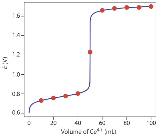
Additional results for this titration curve are shown in Table 9.4.1 and Figure 9.4.1 .
Calculate the titration curve for the titration of 50.0 mL of 0.0500 M Sn2+ with 0.100 M Tl3+. Both the titrand and the titrant are 1.0 M in HCl. The titration reaction is
\[\text{Sn}^{2+}(aq) + \text{Tl}^{3+} \rightleftharpoons \text{Tl}^+(aq) + \text{Sn}^{4+}(aq) \nonumber\]
- Answer
-
The volume of Tl3+ needed to reach the equivalence point is
\[V_{eq} = V_\text{Tl} = \frac{M_\text{Sn}V_\text{Sn}}{M_\text{Tl}} = \frac{(0.050 \text{ M})(50.0 \text{ mL})}{(0.100 \text{ M})} = 25.0 \text{ mL} \nonumber\]
Before the equivalence point, the concentration of unreacted Sn2+ and the concentration of Sn4+ are easy to calculate. For this reason we find the potential using the Nernst equation for the Sn4+/Sn2+ half-reaction. For example, the concentrations of Sn2+ and Sn4+ after adding 10.0 mL of titrant are
\[[\text{Sn}^{2+}] = \frac{(0.050 \text{ M})(50.0 \text{ mL}) - (0.100 \text{ M})(10.0 \text{ mL})}{50.0 \text{ mL} + 10.0 \text{ mL}} = 0.0250 \text{ M} \nonumber\]
\[[\text{Sn}^{4+}] = \frac{(0.100 \text{ M})(10.0 \text{ mL})}{50.0 \text{ mL} + 10.0 \text{ mL}} = 0.0167 \text{ M} \nonumber\]
and the potential is
\[E = +0.139 \text{ V} - \frac{0.05916}{2} \log{\frac{0.0250 \text{ M}}{0.0167 \text{ M}}} = +0.134 \text{ V} \nonumber\]
After the equivalence point, the concentration of Tl+ and the concentration of excess Tl3+ are easy to calculate. For this reason we find the potential using the Nernst equation for the Tl3+/Tl+ half-reaction. For example, after adding 40.0 mL of titrant, the concentrations of Tl+ and Tl3+ are
\[[\text{Tl}^{+}] = \frac{(0.050 \text{ M})(50.0 \text{ mL})}{50.0 \text{ mL} + 40.0 \text{ mL}} = 0.0278 \text{ M} \nonumber\]
\[[\text{Tl}^{3+}] = \frac{(0.100 \text{ M})(40.0 \text{ mL}) - (0.050 \text{ M})(50.0 \text{ mL})}{50.0 \text{ mL} + 40.0 \text{ mL}} = 0.0167 \text{ M} \nonumber\]
and the potential is
\[E = +0.77 \text{ V} - \frac{0.05916}{2} \log{\frac{0.0278 \text{ M}}{0.0167 \text{ M}}} = +0.76 \text{ V} \nonumber\]
At the titration’s equivalence point, the potential, Eeq, potential is
\[E_{eq} = \frac{0.139 \text{ V} + 0.77 \text{ V}}{2} = +0.45 \text{ V} \nonumber\]
Some additional results are shown here.
volume of Tl3+ (mL) E (V) volume of Tl3+ (mL) E (V) 5.00 0.121 30.0 0.75 10.0 0.134 35.0 0.75 15.0 0.144 40.0 0.76 20.0 0.157 45.0 0.76 25.0 0.45
Sketching a Redox Titration Curve
To evaluate the relationship between a titration’s equivalence point and its end point we need to construct only a reasonable approximation of the exact titration curve. In this section we demonstrate a simple method for sketching a redox titration curve. Our goal is to sketch the titration curve quickly, using as few calculations as possible. Let’s use the titration of 50.0 mL of 0.100 M Fe2+ with 0.100 M Ce4+ in a matrix of 1 M HClO4.
This is the same example that we used in developing the calculations for a redox titration curve. You can review the results of that calculation in Table 9.4.1 and Figure 9.4.1 .
We begin by calculating the titration’s equivalence point volume, which, as we determined earlier, is 50.0 mL. Next, we draw our axes, placing the potential, E, on the y-axis and the titrant’s volume on the x-axis. To indicate the equivalence point’s volume, we draw a vertical line that intersects the x-axis at 50.0 mL of Ce4+. Figure 9.4.2 a shows the result of the first step in our sketch.
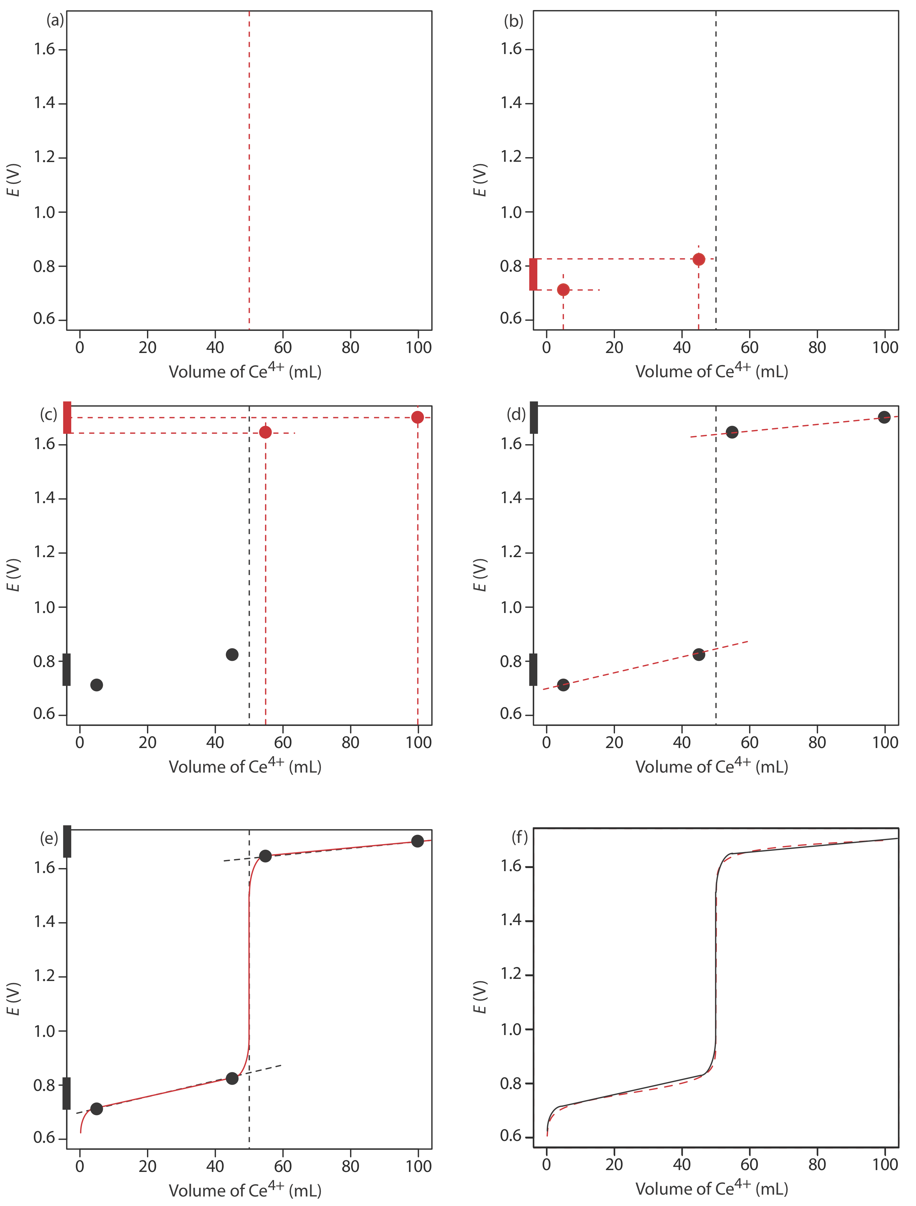
Before the equivalence point, the potential is determined by a redox buffer of Fe2+ and Fe3+. Although we can calculate the potential using the Nernst equation, we can avoid this calculation if we make a simple assumption. You may recall from Chapter 6 that a redox buffer operates over a range of potentials that extends approximately ±(0.05916/n) unit on either side of \(E_{\text{Fe}^{3+}/\text{Fe}^{2+}}^{\circ}\). The potential at the buffer’s lower limit is
\[E = E_{\text{Fe}^{3+}/\text{Fe}^{2+}}^{\circ} - 0.05916 \nonumber\]
when the concentration of Fe2+ is \(10 \times\) greater than that of Fe3+. The buffer reaches its upper potential of
\[E = E_{\text{Fe}^{3+}/\text{Fe}^{2+}}^{\circ} + 0.05916 \nonumber\]
when the concentration of Fe2+ is \(10 \times\) smaller than that of Fe3+. The redox buffer spans a range of volumes from approximately 10% of the equivalence point volume to approximately 90% of the equivalence point volume. Figure 9.4.2 b shows the second step in our sketch. First, we superimpose a ladder diagram for Fe on the y-axis, using its \(E_{\text{Fe}^{3+}/\text{Fe}^{2+}}^{\circ}\) value of 0.767 V and including the buffer’s range of potentials. Next, we add points for the potential at 10% of Veq (a potential of 0.708 V at 5.0 mL) and for the potential at 90% of Veq (a potential of 0.826 V at 45.0 mL).
We used a similar approach when sketching the acid–base titration curve for the titration of acetic acid with NaOH; see Chapter 9.2 for details.
The third step in sketching our titration curve is to add two points after the equivalence point. Here the potential is controlled by a redox buffer of Ce3+ and Ce4+. The redox buffer is at its lower limit of
\[E = E_{\text{Ce}^{4+}/\text{Ce}^{3+}}^{\circ} - 0.05916 \nonumber\]
when the titrant reaches 110% of the equivalence point volume and the potential is \(E_{\text{Ce}^{4+}/\text{Ce}^{3+}}^{\circ}\) when the volume of Ce is \(2 \times V_{eq}\).
We used a similar approach when sketching the complexation titration curve for the titration of Mg2+ with EDTA; see Chapter 9.3 for details.
Figure 9.4.2 c shows the third step in our sketch. First, we superimpose a ladder diagram for Ce on the y-axis, using its \(E_{\text{Ce}^{4+}/\text{Ce}^{3+}}^{\circ}\) value of 1.70 V and including the buffer’s range. Next, we add points representing the potential at 110% of Veq (a value of 1.66 V at 55.0 mL) and at 200% of Veq (a value of 1.70 V at 100.0 mL).
Next, we draw a straight line through each pair of points, extending the line through the vertical line that indicates the equivalence point’s volume (Figure 9.4.2 d). Finally, we complete our sketch by drawing a smooth curve that connects the three straight-line segments (Figure 9.4.2 e). A comparison of our sketch to the exact titration curve (Figure 9.4.2 f) shows that they are in close agreement.
Sketch the titration curve for the titration of 50.0 mL of 0.0500 M Sn4+ with 0.100 M Tl+. Both the titrand and the titrant are 1.0 M in HCl. The titration reaction is
\[\text{Sn}^{2+}(aq) + \text{Tl}^{3+}(aq) \rightleftharpoons \text{Tl}^{+}(aq) + \text{Sn}^{4+}(aq) \nonumber\]
Compare your sketch to your calculated titration curve from Exercise 9.4.1 .
- Answer
-
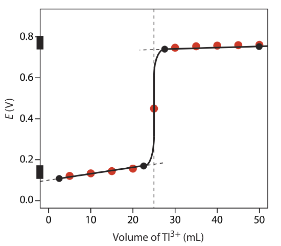
The figure below shows a sketch of the titration curve. The two points before the equivalence point
VTl = 2.5 mL, E = +0.109 V and VTl = 22.5 mL, E = +0.169 V
are plotted using the redox buffer for Sn4+/Sn2+, which spans a potential range of +0.139 ± 0.5916/2. The two points after the equivalence point
VTl = 27.5 mL, E = +0.74 V and VTl = 50 mL, E = +0.77 V
are plotted using the redox buffer for Tl3+/Tl+, which spans the potential range of +0.139 ± 0.5916/2. The black dots and curve are the approximate sketch of the titration curve. The points in red are the calculations from Exercise 9.4.1 .
Selecting and Evaluating the End Point
A redox titration’s equivalence point occurs when we react stoichiometrically equivalent amounts of titrand and titrant. As is the case for acid–base titrations and complexation titrations, we estimate the equivalence point of a redox titration using an experimental end point. A variety of methods are available for locating a redox titration’s end point, including indicators and sensors that respond to a change in the solution conditions.
Where is the Equivalence Point
For an acid–base titration or a complexometric titration the equivalence point is almost identical to the inflection point on the steeply rising part of the titration curve. If you look back at Figure 9.2.2 and Figure 9.3.3, you will see that the inflection point is in the middle of this steep rise in the titration curve, which makes it relatively easy to find the equivalence point when you sketch these titration curves. We call this a symmetric equivalence point. If the stoichiometry of a redox titration is 1:1—that is, one mole of titrant reacts with each mole of titrand—then the equivalence point is symmetric. If the titration reaction’s stoichiometry is not 1:1, then the equivalence point is closer to the top or to the bottom of the titration curve’s sharp rise. In this case we have an asymmetric equivalence point.
Derive a general equation for the equivalence point’s potential when titrating Fe2+ with \(\text{MnO}_4^-\).
\[5\text{Fe}^{2+}(aq) + \text{MnO}_4^-(aq) + 8\text{H}^+(aq) \rightarrow 5\text{Fe}^{3+}(aq) + \text{Mn}^{2+}(aq) + 4\text{H}_2\text{O}(l) \nonumber\]
Solution
The half-reactions for the oxidation of Fe2+ and the reduction of \(\text{MnO}_4^-\) are
\[\text{Fe}^{2+}(aq) \rightarrow \text{Fe}^{3+}(aq) + e^- \nonumber\]
\[\text{MnO}_4^-(aq) + 8\text{H}^+(aq) + 5 e^- \rightarrow \text{Mn}^{2+}(aq) + 4\text{H}_2\text{O}(l) \nonumber\]
for which the Nernst equations are
\[E = E_{\text{Fe}^{3+}/\text{Fe}^{2+}}^{\circ} - 0.5916 \log{\frac{[\text{Fe}^{2+}]}{[\text{Fe}^{3+}]}} \nonumber\]
\[E = E_{\text{MnO}_4^{-}/\text{Mn}^{2+}}^{\circ} - \frac{0.5916}{5} \log{\frac{[\text{Mn}^{2+}]}{[\text{MnO}_4^{-}][\text{H}^+]^8}} \nonumber\]
Before we add together these two equations we must multiply the second equation by 5 so that we can combine the log terms; thus
\[6E_{eq} = E_{\text{Fe}^{3+}/\text{Fe}^{2+}}^{\circ} + 5E_{\text{MnO}_4^{-}/\text{Mn}^{2+}}^{\circ} - 0.05916 \log{\frac{[\text{Fe}^{2+}][\text{Mn}^{2+}]}{[\text{Fe}^{3+}][\text{MnO}_4^{-}][\text{H}^+]^8}} \nonumber\]
At the equivalance point we know that
\[[\text{Fe}^{2+}] = 5 \times [\text{MnO}_4^-] \text{ and } [\text{Fe}^{3+}] = 5 \times [\text{Mn}^{2+}] \nonumber\]
Substituting these equalities into the previous equation and rearranging gives us a general equation for the potential at the equivalence point.
\[6E_{eq} = E_{\text{Fe}^{3+}/\text{Fe}^{2+}}^{\circ} + 5E_{\text{MnO}_4^{-}/\text{Mn}^{2+}}^{\circ} - 0.05916 \log{\frac{5[\text{MnO}_4^{-}][\text{Mn}^{2+}]}{5[\text{Mn}^{2+}][\text{MnO}_4^{-}][\text{H}^+]^8}} \nonumber\]
\[E_{eq} = \frac{E_{\text{Fe}^{3+}/\text{Fe}^{2+}}^{\circ} + 5E_{\text{MnO}_4^{-}/\text{Mn}^{2+}}^{\circ}}{6} - \frac{0.05916}{6} \log{\frac{1}{[\text{H}^+]^8}} \nonumber\]
\[E_{eq} = \frac{E_{\text{Fe}^{3+}/\text{Fe}^{2+}}^{\circ} + 5E_{\text{MnO}_4^{-}/\text{Mn}^{2+}}^{\circ}}{6} + \frac{0.05916 \times 8}{6} \log{[\text{H}^+]} \nonumber\]
\[E_{eq} = \frac{E_{\text{Fe}^{3+}/\text{Fe}^{2+}}^{\circ} + 5E_{\text{MnO}_4^{-}/\text{Mn}^{2+}}^{\circ}}{6} - 0.07888 \text{pH} \nonumber\]
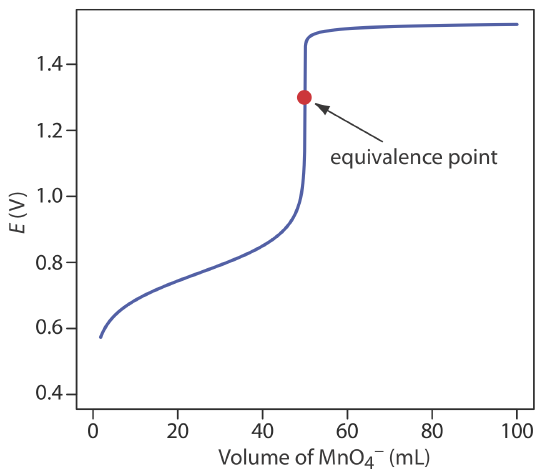
Our equation for the equivalence point has two terms. The first term is a weighted average of the titrand’s and the titrant’s standard state potentials, in which the weighting factors are the number of electrons in their respective half-reactions. The second term shows that Eeq for this titration is pH-dependent. At a pH of 1 (in H2SO4), for example, the equivalence point has a potential of
\[E_{eq} = \frac{0.768 + 5 \times 1.51}{6} - 0.07888 \times 1 = 1.31 \text{ V} \nonumber\]
Figure 9.4.3 shows a typical titration curve for titration of Fe2+ with \(\text{MnO}_4^-\). Note that the titration’s equivalence point is asymmetrical.
Derive a general equation for the equivalence point’s potential for the titration of U4+ with Ce4+. The unbalanced reaction is
\[\text{Ce}^{4+}(aq) + \text{U}^{4+}(aq) \rightarrow \text{UO}_2^{2+}(aq) + \text{Ce}^{3+}(aq) \nonumber\]
What is the equivalence point’s potential if the pH is 1?
- Answer
-
The two half reactions are
\[\text{Ce}^{4+}(aq) + e^- \rightarrow \text{Ce}^{3+}(aq) \nonumber\]
\[\text{U}^{4+}(aq) +2\text{H}_2\text{O}(l) \rightarrow \text{UO}_2^{2+}(aq)) + 4\text{H}^+(aq) +2e^- \nonumber\]
for which the Nernst equations are
\[E = E_{\text{Ce}^{4+}/\text{Ce}^{3+}}^{\circ} - 0.05916 \log{\frac{[\text{Ce}^{3+}]}{[\text{Ce}^{4+}]}} \nonumber\]
\[E = E_{\text{UO}_2^{2+}/\text{U}^{4+}}^{\circ} - \frac{0.05916}{2} \log{\frac{[\text{U}^{4+}]}{[\text{UO}_2^{2+}][\text{H}^+]^4}} \nonumber\]
Before adding these two equations together we must multiply the second equation by 2 so that we can combine the log terms; thus
\[3E = E_{\text{Ce}^{4+}/\text{Ce}^{3+}}^{\circ} + 2E_{\text{UO}_2^{2+}/\text{U}^{4+}}^{\circ} - 0.05916 \log{\frac{[\text{Ce}^{3+}][\text{U}^{4+}]}{[\text{Ce}^{4+}][\text{UO}_2^{2+}][\text{H}^+]^4}} \nonumber\]
At the equivalence point we know that
\[[\text{Ce}^{3+}] = 2 \times [\text{UO}_2^{2+}] \text{ and } [\text{Ce}^{4+}] = 2 \times [\text{U}^{4+}] \nonumber\]
Substituting these equalities into the previous equation and rearranging gives us a general equation for the potential at the equivalence point.
\[3E = E_{\text{Ce}^{4+}/\text{Ce}^{3+}}^{\circ} + 2E_{\text{UO}_2^{2+}/\text{U}^{4+}}^{\circ} - 0.05916 \log{\frac{2[\text{UO}_2^{2+}][\text{U}^{4+}]}{2[\text{U}^{4+}][\text{UO}_2^{2+}][\text{H}^+]^4}} \nonumber\]
\[E = \frac{E_{\text{Ce}^{4+}/\text{Ce}^{3+}}^{\circ} + 2E_{\text{UO}_2^{2+}/\text{U}^{4+}}^{\circ}}{3} - \frac{0.05916}{3} \log{\frac{1}{[\text{H}^+]^4}} \nonumber\]
\[E = \frac{E_{\text{Ce}^{4+}/\text{Ce}^{3+}}^{\circ} + 2E_{\text{UO}_2^{2+}/\text{U}^{4+}}^{\circ}}{3} + \frac{0.05916 \times 4}{3} \log{[\text{H}^+]^4} \nonumber\]
\[E = \frac{E_{\text{Ce}^{4+}/\text{Ce}^{3+}}^{\circ} + 2E_{\text{UO}_2^{2+}/\text{U}^{4+}}^{\circ}}{3} - 0.07888\text{pH} \nonumber\]
At a pH of 1 the equivalence point has a potential of
\[E = \frac{1.72 + 2 \times 0.327}{3} - 0.07888 \times 1 = +0.712 \text{ V} \nonumber\]
Finding the End Point With an Indicator
Three types of indicators are used to signal a redox titration’s end point. The oxidized and reduced forms of some titrants, such as \(\text{MnO}_4^-\), have different colors. A solution of \(\text{MnO}_4^-\) is intensely purple. In an acidic solution, however, permanganate’s reduced form, Mn2+, is nearly colorless. When using \(\text{MnO}_4^-\) as a titrant, the titrand’s solution remains colorless until the equivalence point. The first drop of excess \(\text{MnO}_4^-\) produces a permanent tinge of purple, signaling the end point.
Some indicators form a colored compound with a specific oxidized or reduced form of the titrant or the titrand. Starch, for example, forms a dark purple complex with \(\text{I}_3^-\). We can use this distinct color to signal the presence of excess \(\text{I}_3^-\) as a titrant—a change in color from colorless to purple—or the completion of a reaction that consumes \(\text{I}_3^-\) as the titrand— a change in color from purple to colorless. Another example of a specific indicator is thiocyanate, SCN–, which forms the soluble red-colored complex of Fe(SCN)2+ in the presence of Fe3+.
The most important class of indicators are substances that do not participate in the redox titration, but whose oxidized and reduced forms differ in color. When we add a redox indicator to the titrand, the indicator imparts a color that depends on the solution’s potential. As the solution’s potential changes with the addition of titrant, the indicator eventually changes oxidation state and changes color, signaling the end point.
To understand the relationship between potential and an indicator’s color, consider its reduction half-reaction
\[\text{In}_\text{ox} + ne^- \rightleftharpoons \text{In}_\text{red} \nonumber\]
where Inox and Inred are, respectively, the indicator’s oxidized and reduced forms.
For simplicity, Inox and Inred are shown without specific charges. Because there is a change in oxidation state, Inox and Inred cannot both be neutral.
The Nernst equation for this half-reaction is
\[E = E_{\text{In}_\text{ox}/\text{In}_\text{red}}^{\circ} - \frac{0.05916}{n} \log{\frac{[\text{In}_\text{red}]}{[\text{In}_\text{ox}]}} \nonumber\]
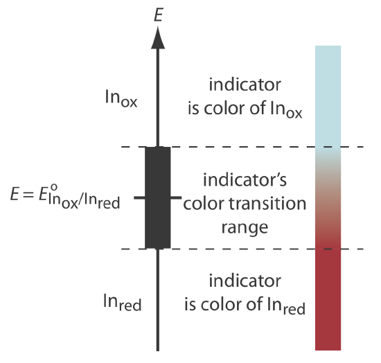
As shown in Figure 9.4.4 , if we assume the indicator’s color changes from that of Inox to that of Inred when the ratio [Inred]/[Inox] changes from 0.1 to 10, then the end point occurs when the solution’s potential is within the range
\[E = E_{\text{In}_\text{ox}/\text{In}_\text{red}}^{\circ} \pm \frac{0.05916}{n} \nonumber\]
This is the same approach we took in considering acid–base indicators and complexation indicators.
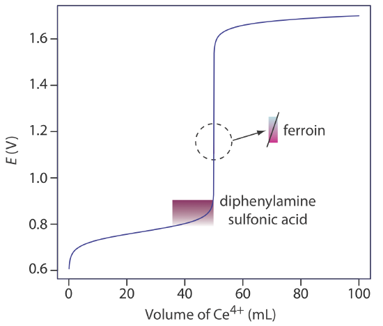
A partial list of redox indicators is shown in Table 9.4.2 . Examples of an appropriate and an inappropriate indicator for the titration of Fe2+ with Ce4+ are shown in Figure 9.4.5 .
Other Methods for Finding the End Point
Another method for locating a redox titration’s end point is a potentiometric titration in which we monitor the change in potential while we add the titrant to the titrand. The end point is found by examining visually the titration curve. The simplest experimental design for a potentiometric titration consists of a Pt indicator electrode whose potential is governed by the titrand’s or the titrant’s redox half-reaction, and a reference electrode that has a fixed potential. Other methods for locating the titration’s end point include thermometric titrations and spectrophotometric titrations.
You will a further discussion of potentiometry in Chapter 11.
Representative Method 9.4.1: Determination of Total Chlorine Residual
The best way to appreciate the theoretical and the practical details discussed in this section is to carefully examine a typical redox titrimetric method. Although each method is unique, the following description of the determination of the total chlorine residual in water provides an instructive example of a typical procedure. The description here is based on Method 4500-Cl B as published in Standard Methods for the Examination of Water and Wastewater, 20th Ed., American Public Health Association: Washington, D. C., 1998.
Description of the Method
The chlorination of a public water supply produces several chlorine-containing species, the combined concentration of which is called the total chlorine residual. Chlorine is present in a variety of chemical states, including the free residual chlorine, which consists of Cl2, HOCl and OCl–, and the combined chlorine residual, which consists of NH2Cl, NHCl2, and NCl3. The total chlorine residual is determined by using the oxidizing power of chlorine to convert I– to \(\text{I}_3^-\). The amount of \(\text{I}_3^-\) formed is then determined by titrating with Na2S2O3 using starch as an indicator. Regardless of its form, the total chlorine residual is reported as if Cl2 is the only source of chlorine, and is reported as mg Cl/L.
Procedure
Select a volume of sample that requires less than 20 mL of Na2S2O3 to reach the end point. Using glacial acetic acid, acidify the sample to a pH between 3 and 4, and add about 1 gram of KI. Titrate with Na2S2O3 until the yellow color of \(\text{I}_3^-\) begins to disappear. Add 1 mL of a starch indicator solution and continue titrating until the blue color of the starch–\(\text{I}_3^-\) complex disappears (Figure 9.4.6 ). Use a blank titration to correct the volume of titrant needed to reach the end point for reagent impurities.

Questions
1. Is this an example of a direct or an indirect analysis?
This is an indirect analysis because the chlorine-containing species do not react with the titrant. Instead, the total chlorine residual oxidizes I– to \(\text{I}_3^-\), and the amount of \(\text{I}_3^-\) is determined by titrating with Na2S2O3.
2. Why does the procedure rely on an indirect analysis instead of directly titrating the chlorine-containing species using KI as a titrant?
Because the total chlorine residual consists of six different species, a titration with I– does not have a single, well-defined equivalence point. By converting the chlorine residual to an equivalent amount of \(\text{I}_3^-\), the indirect titration with Na2S2O3 has a single, useful equivalence point. Even if the total chlorine residual is from a single species, such as HOCl, a direct titration with KI is impractical. Because the product of the titration, \(\text{I}_3^-\), imparts a yellow color, the titrand’s color would change with each addition of titrant, making it difficult to find a suitable indicator.
3. Both oxidizing and reducing agents can interfere with this analysis. Explain the effect of each type of interferent on the total chlorine residual.
An interferent that is an oxidizing agent converts additional I– to \(\text{I}_3^-\). Because this extra \(\text{I}_3^-\) requires an additional volume of Na2S2O3 to reach the end point, we overestimate the total chlorine residual. If the interferent is a reducing agent, it reduces back to I– some of the \(\text{I}_3^-\) produced by the reaction between the total chlorine residual and iodide; as a result, we underestimate the total chlorine residual.
Quantitative Applications
Although many quantitative applications of redox titrimetry have been re- placed by other analytical methods, a few important applications continue to find relevance. In this section we review the general application of redox titrimetry with an emphasis on environmental, pharmaceutical, and industrial applications. We begin, however, with a brief discussion of selecting and characterizing redox titrants, and methods for controlling the titrand’s oxidation state.
Adjusting the Titrand's Oxidation State
If a redox titration is to be used in a quantitative analysis, the titrand initially must be present in a single oxidation state. For example, iron is determined by a redox titration in which Ce4+ oxidizes Fe2+ to Fe3+. Depending on the sample and the method of sample preparation, iron initially may be present in both the +2 and +3 oxidation states. Before titrating, we must reduce any Fe3+ to Fe2+ if we want to determine the total concentration of iron in the sample. This type of pretreatment is accomplished using an auxiliary reducing agent or oxidizing agent.
A metal that is easy to oxidize—such as Zn, Al, and Ag—can serve as an auxiliary reducing agent. The metal, as a coiled wire or powder, is added to the sample where it reduces the titrand. Because any unreacted auxiliary reducing agent will react with the titrant, it is removed before we begin the titration by removing the coiled wire or by filtering.
An alternative method for using an auxiliary reducing agent is to immobilize it in a column. To prepare a reduction column an aqueous slurry of the finally divided metal is packed in a glass tube equipped with a porous plug at the bottom. The sample is placed at the top of the column and moves through the column under the influence of gravity or vacuum suction. The length of the reduction column and the flow rate are selected to ensure the analyte’s complete reduction.
Two common reduction columns are used. In the Jones reductor the column is filled with amalgamated zinc, Zn(Hg), which is prepared by briefly placing Zn granules in a solution of HgCl2. Oxidation of zinc
\[\text{Zn(Hg)}(s) \rightarrow \text{Zn}^{2+}(aq) + \text{Hg}(l) + 2e^- \nonumber\]
provides the electrons for reducing the titrand. In the Walden reductor the column is filled with granular Ag metal. The solution containing the titrand is acidified with HCl and passed through the column where the oxidation of silver
\[\text{Ag}(s) + \text{Cl}^- (aq) \rightarrow \text{AgCl}(s) + e^- \nonumber\]
provides the necessary electrons for reducing the titrand. Table 9.4.3 provides a summary of several applications of reduction columns.
Several reagents are used as auxiliary oxidizing agents, including ammonium peroxydisulfate, (NH4)2S2O8, and hydrogen peroxide, H2O2. Peroxydisulfate is a powerful oxidizing agent
\[\text{S}_2\text{O}_8^{2-}(aq) + 2e^- \rightarrow 2\text{SO}_4^{2-}(aq) \nonumber\]
that is capable of oxidizing Mn2+ to \(\text{MnO}_4^-\), Cr3+ to \(\text{Cr}_2\text{O}_7^{2-}\), and Ce3+ to Ce4+. Excess peroxydisulfate is destroyed by briefly boiling the solution. The reduction of hydrogen peroxide in an acidic solution
\[\text{H}_2\text{O}_2(aq) + 2\text{H}^+(aq) + 2e^- \rightarrow 2\text{H}_2\text{O}(l) \nonumber\]
provides another method for oxidizing a titrand. Excess H2O2 is destroyed by briefly boiling the solution.
Selecting and Standardizing a Titrant
If it is to be used quantitatively, the titrant’s concentration must remain stable during the analysis. Because a titrant in a reduced state is susceptible to air oxidation, most redox titrations use an oxidizing agent as the titrant. There are several common oxidizing titrants, including \(\text{MnO}_4^-\), Ce4+, \(\text{Cr}_2\text{O}_7^{2-}\), and \(\text{I}_3^-\). Which titrant is used often depends on how easily it oxidizes the titrand. A titrand that is a weak reducing agent needs a strong oxidizing titrant if the titration reaction is to have a suitable end point.
The two strongest oxidizing titrants are \(\text{MnO}_4^-\) and Ce4+, for which the reduction half-reactions are
\[\text{MnO}_4^-(aq) + 8\text{H}^+(aq) + 5e^- \rightleftharpoons \text{Mn}^{2+}(aq) + 4\text{H}_2\text{O}(l) \nonumber\]
\[\text{Ce}^{4+}(aq) + e^- \rightleftharpoons \text{Ce}^{3+}(aq) \nonumber\]
A solution of Ce4+ in 1 M H2SO4 usually is prepared from the primary standard cerium ammonium nitrate, Ce(NO3)4•2NH4NO3. When prepared using a reagent grade material, such as Ce(OH)4, the solution is standardized against a primary standard reducing agent such as Na2C2O4 or Fe2+ (prepared from iron wire) using ferroin as an indicator. Despite its availability as a primary standard and its ease of preparation, Ce4+ is not used as frequently as \(\text{MnO}_4^-\) because it is more expensive.
The standardization reactions are
\[\text{Ce}^{4+}(aq) + \text{Fe}^{2+}(aq) \rightarrow \text{Fe}^{3+}(aq) + \text{Ce}^{3+}(aq) \nonumber\]
\[2\text{Ce}^{4+}(aq) + \text{H}_2\text{C}_2\text{O}_4(aq) \rightarrow 2\text{Ce}^{3+}(aq) + 2\text{CO}_2(g) + 2\text{H}^+(aq) \nonumber\]
A solution of \(\text{MnO}_4^-\) is prepared from KMnO4, which is not available as a primary standard. An aqueous solution of permanganate is thermodynamically unstable due to its ability to oxidize water.
\[4\text{MnO}_4^-(aq) + 2\text{H}_2\text{O}(l) \rightleftharpoons 4\text{MnO}_2(s) + 3\text{O}_2 (g) + 4\text{OH}^-(aq) \nonumber\]
This reaction is catalyzed by the presence of MnO2, Mn2+, heat, light, and the presence of acids and bases. A moderately stable solution of permanganate is prepared by boiling it for an hour and filtering through a sintered glass filter to remove any solid MnO2 that precipitates. Standardization is accomplished against a primary standard reducing agent such as Na2C2O4 or Fe2+ (prepared from iron wire), with the pink color of excess \(\text{MnO}_4^-\) signaling the end point. A solution of \(\text{MnO}_4^-\) prepared in this fashion is stable for 1–2 weeks, although you should recheck the standardization periodically.
The standardization reactions are
\[\text{MnO}_4^-(aq) + 5\text{Fe}^{2+}(aq) + 8\text{H}^+(aq) \rightarrow \text{Mn}^{2+}(aq) + 5\text{Fe}^{3+}(aq) + 4\text{H}_2\text{O}(l) \nonumber\]
\[2\text{MnO}_4^-(aq) + 5\text{H}_2\text{C}_2\text{O}_4(aq) + 6\text{H}^+(aq) \rightarrow 2\text{Mn}^{2+}(aq) + 10\text{CO}_2(g) + 8\text{H}_2\text{O}(l) \nonumber\]
Potassium dichromate is a relatively strong oxidizing agent whose principal advantages are its availability as a primary standard and its long term stability when in solution. It is not, however, as strong an oxidizing agent as \(\text{MnO}_4^-\) or Ce4+, which makes it less useful when the titrand is a weak reducing agent. Its reduction half-reaction is
\[\text{Cr}_2\text{O}_7^{2-}(aq) + 14\text{H}^+(aq) + 6e^- \rightleftharpoons 2\text{Cr}^{3+}(aq) + 7\text{H}_2\text{O}(l) \nonumber\]
Although a solution of \(\text{Cr}_2\text{O}_7^{2-}\) is orange and a solution of Cr3+ is green, neither color is intense enough to serve as a useful indicator. Diphenylamine sulfonic acid, whose oxidized form is red-violet and reduced form is colorless, gives a very distinct end point signal with \(\text{Cr}_2\text{O}_7^{2-}\).
Iodine is another important oxidizing titrant. Because it is a weaker oxidizing agent than \(\text{MnO}_4^-\), Ce4+, and \(\text{Cr}_2\text{O}_7^{2-}\), it is useful only when the titrand is a stronger reducing agent. This apparent limitation, however, makes I2 a more selective titrant for the analysis of a strong reducing agent in the presence of a weaker reducing agent. The reduction half-reaction for I2 is
\[\text{I}_2(aq) + 2e^- \rightleftharpoons 2\text{I}^-(aq) \nonumber\]
Because iodine is not very soluble in water, solutions are prepared by adding an excess of I–. The complexation reaction
\[\text{I}_2(aq) + \text{I}^-(aq) \rightleftharpoons \text{I}_3^-(aq) \nonumber\]
increases the solubility of I2 by forming the more soluble triiodide ion, \(\text{I}_3^-\). Even though iodine is present as \(\text{I}_3^-\) instead of I2, the number of electrons in the reduction half-reaction is unaffected.
\[\text{I}_3^-(aq) + 2e^-(aq) \rightleftharpoons 3\text{I}^-(aq) \nonumber\]
Solutions of \(\text{I}_3^-\) normally are standardized against Na2S2O3 using starch as a specific indicator for \(\text{I}_3^-\).
The standardization reaction is
\[\text{I}_3^-(aq) + 2\text{S}_2\text{O}_3^{2-}(aq) \rightarrow 3\text{I}^-(aq) + 2\text{S}_4\text{O}_6^{2-} (aq) \nonumber\]
An oxidizing titrant such as \(\text{MnO}_4^-\), Ce4+, \(\text{Cr}_2\text{O}_7^{2-}\), and \(\text{I}_3^-\), is used when the titrand is in a reduced state. If the titrand is in an oxidized state, we can first reduce it with an auxiliary reducing agent and then complete the titration using an oxidizing titrant. Alternatively, we can titrate it using a reducing titrant. Iodide is a relatively strong reducing agent that could serve as a reducing titrant except that its solutions are susceptible to the air-oxidation of I– to \(\text{I}_3^-\).
\[3\text{I}^-(aq) \rightleftharpoons \text{I}_3^- (aq) + 2e^- \nonumber\]
A freshly prepared solution of KI is clear, but after a few days it may show a faint yellow coloring due to the presence of \(\text{I}_3^-\).
Instead, adding an excess of KI reduces the titrand and releases a stoichiometric amount of \(\text{I}_3^-\). The amount of \(\text{I}_3^-\) produced is then determined by a back titration using thiosulfate, \(\text{S}_2\text{O}_3^{2-}\), as a reducing titrant.
\[2\text{S}_2\text{O}_3^{2-}(aq) \rightleftharpoons \text{S}_4\text{O}_6^{2-}(aq) + 2e^- \nonumber\]
Solutions of \(\text{S}_2\text{O}_3^{2-}\) are prepared using Na2S2O3•5H2O and are standardized before use. Standardization is accomplished by dissolving a carefully weighed portion of the primary standard KIO3 in an acidic solution that contains an excess of KI. The reaction between \(\text{IO}_3^-\) and I–
\[\text{IO}_3^-(aq) + 8\text{I}^-(aq) + 6\text{H}^+(aq) \rightarrow 3\text{I}_3^-(aq) + 3\text{H}_2\text{O}(l) \nonumber\]
liberates a stoichiometric amount of I-3 . By titrating this \(\text{I}_3^-\) with thiosulfate, using starch as a visual indicator, we can determine the concentration of \(\text{S}_2\text{O}_3^{2-}\) in the titrant.
The standardization titration is
\[\text{I}_3^-(aq) + 2\text{S}_2\text{O}_3^{2-}(aq) \rightarrow 3\text{I}^-(aq) + \text{S}_4\text{O}_6^{2-}(aq) \nonumber\]
which is the same reaction used to standardize solutions of \(\text{I}_3^-\). This approach to standardizing solutions of \(\text{S}_2\text{O}_2^{3-}\) is similar to that used in the determination of the total chlorine residual outlined in Representative Method 9.4.1.
Although thiosulfate is one of the few reducing titrants that is not readily oxidized by contact with air, it is subject to a slow decomposition to bisulfite and elemental sulfur. If used over a period of several weeks, a solution of thiosulfate is restandardized periodically. Several forms of bacteria are able to metabolize thiosulfate, which leads to a change in its concentration. This problem is minimized by adding a preservative such as HgI2 to the solution.
Another useful reducing titrant is ferrous ammonium sulfate, Fe(NH4)2(SO4)2•6H2O, in which iron is present in the +2 oxidation state. A solution of Fe2+ is susceptible to air-oxidation, but when prepared in 0.5 M H2SO4 it remains stable for as long as a month. Periodic restandardization with K2Cr2O7 is advisable. Ferrous ammonium sulfate is used as the titrant in a direct analysis of the titrand, or, it is added to the titrand in excess and the amount of Fe3+ produced determined by back titrating with a standard solution of Ce4+ or \(\text{Cr}_2\text{O}_7^{2-}\).
Inorganic Analysis
One of the most important applications of redox titrimetry is evaluating the chlorination of public water supplies. Representative Method 9.4.1, for example, describes an approach for determining the total chlorine residual using the oxidizing power of chlorine to oxidize I– to \(\text{I}_3^-\). The amount of \(\text{I}_3^-\) is determined by back titrating with \(\text{S}_2\text{O}_3^{2-}\).
The efficiency of chlorination depends on the form of the chlorinating species. There are two contributions to the total chlorine residual—the free chlorine residual and the combined chlorine residual. The free chlorine residual includes forms of chlorine that are available for disinfecting the water supply. Examples of species that contribute to the free chlorine residual include Cl2, HOCl and OCl–. The combined chlorine residual includes those species in which chlorine is in its reduced form and, therefore, no longer capable of providing disinfection. Species that contribute to the combined chlorine residual are NH2Cl, NHCl2 and NCl3.
When a sample of iodide-free chlorinated water is mixed with an excess of the indicator N,N-diethyl-p-phenylenediamine (DPD), the free chlorine oxidizes a stoichiometric portion of DPD to its red-colored form. The oxidized DPD is then back-titrated to its colorless form using ferrous ammonium sulfate as the titrant. The volume of titrant is proportional to the free residual chlorine.
Having determined the free chlorine residual in the water sample, a small amount of KI is added, which catalyzes the reduction of monochloramine, NH2Cl, and oxidizes a portion of the DPD back to its red-colored form. Titrating the oxidized DPD with ferrous ammonium sulfate yields the amount of NH2Cl in the sample. The amount of dichloramine and trichloramine are determined in a similar fashion.
The methods described above for determining the total, free, or combined chlorine residual also are used to establish a water supply’s chlorine demand. Chlorine demand is defined as the quantity of chlorine needed to react completely with any substance that can be oxidized by chlorine, while also maintaining the desired chlorine residual. It is determined by adding progressively greater amounts of chlorine to a set of samples drawn from the water supply and determining the total, free, or combined chlorine residual.
Another important example of redox titrimetry, which finds applications in both public health and environmental analysis, is the determination of dissolved oxygen. In natural waters, such as lakes and rivers, the level of dissolved O2 is important for two reasons: it is the most readily available oxidant for the biological oxidation of inorganic and organic pollutants; and it is necessary for the support of aquatic life. In a wastewater treatment plant dissolved O2 is essential for the aerobic oxidation of waste materials. If the concentration of dissolved O2 falls below a critical value, aerobic bacteria are replaced by anaerobic bacteria, and the oxidation of organic waste produces undesirable gases, such as CH4 and H2S.
One standard method for determining dissolved O2 in natural waters and wastewaters is the Winkler method. A sample of water is collected without exposing it to the atmosphere, which might change the concentration of dissolved O2. The sample first is treated with a solution of MnSO4 and then with a solution of NaOH and KI. Under these alkaline conditions the dissolved oxygen oxidizes Mn2+ to MnO2.
\[2\text{Mn}^{2+}(aq) + 4\text{OH}^-(aq) + \text{O}_2(g) \rightarrow 2\text{MnO}_2(s) + 2\text{H}_2\text{O}(l) \nonumber\]
After the reaction is complete, the solution is acidified with H2SO4. Under the now acidic conditions, I– is oxidized to \(\text{I}_3^-\) by MnO2.
\[\text{MnO}_2(s) + 3\text{I}^-(aq) + 4\text{H}^+(aq) \rightarrow \text{Mn}^{2+}(aq) + \text{I}_3^-(aq) + 2\text{H}_2\text{O}(l) \nonumber\]
The amount of \(\text{I}_3^-\) that forms is determined by titrating with \(\text{S}_2\text{O}_3^{2-}\) using starch as an indicator. The Winkler method is subject to a variety of interferences and several modifications to the original procedure have been proposed. For example, \(\text{NO}_2^-\) interferes because it reduces \(\text{I}_3^-\) to I– under acidic conditions. This interference is eliminated by adding sodium azide, NaN3, which reduces \(\text{NO}_2^-\) to N2. Other reducing agents, such as Fe2+, are eliminated by pretreating the sample with KMnO4 and destroying any excess permanganate with K2C2O4.
Another important example of redox titrimetry is the determination of water in nonaqueous solvents. The titrant for this analysis is known as the Karl Fischer reagent and consists of a mixture of iodine, sulfur dioxide, pyridine, and methanol. Because the concentration of pyridine is sufficiently large, I2 and SO2 react with pyridine (py) to form the complexes py•I2 and py•SO2. When added to a sample that contains water, I2 is reduced to I– and SO2 is oxidized to SO3.
\[\text{py}\cdot\text{I}_2 + \text{py}\cdot\text{SO}_2 + \text{H}_2\text{O} + 2\text{py} \rightarrow 2\text{py}\cdot\text{HI} + \text{py}\cdot\text{SO}_3 \nonumber\]
Methanol is included to prevent the further reaction of py•SO3 with water. The titration’s end point is signaled when the solution changes from the product’s yellow color to the brown color of the Karl Fischer reagent.
Organic Analysis
Redox titrimetry also is used for the analysis of organic analytes. One important example is the determination of the chemical oxygen demand (COD) of natural waters and wastewaters. The COD is a measure of the quantity of oxygen necessary to oxidize completely all the organic matter in a sample to CO2 and H2O. Because no attempt is made to correct for organic matter that is decomposed biologically, or for slow decomposition kinetics, the COD always overestimates a sample’s true oxygen demand. The determination of COD is particularly important in the management of industrial wastewater treatment facilities where it is used to monitor the release of organic-rich wastes into municipal sewer systems or into the environment.
A sample’s COD is determined by refluxing it in the presence of excess K2Cr2O7, which serves as the oxidizing agent. The solution is acidified with H2SO4, using Ag2SO4 to catalyze the oxidation of low molecular weight fatty acids. Mercuric sulfate, HgSO4, is added to complex any chloride that is present, which prevents the precipitation of the Ag+ catalyst as AgCl. Under these conditions, the efficiency for oxidizing organic matter is 95–100%. After refluxing for two hours, the solution is cooled to room temperature and the excess \(\text{Cr}_2\text{O}_7^{2-}\) determined by a back titration using ferrous ammonium sulfate as the titrant and ferroin as the indicator. Because it is difficult to remove completely all traces of organic matter from the reagents, a blank titration is performed. The difference in the amount of ferrous ammonium sulfate needed to titrate the sample and the blank is proportional to the COD.
Iodine has been used as an oxidizing titrant for a number of compounds of pharmaceutical interest. Earlier we noted that the reaction of \(\text{S}_2\text{O}_3^{2-}\) with \(\text{I}_3^-\) produces the tetrathionate ion, \(\text{S}_4\text{O}_6^{2-}\). The tetrathionate ion is actually a dimer that consists of two thiosulfate ions connected through a disulfide (–S–S–) linkage. In the same fashion, \(\text{I}_3^-\) is used to titrate mercaptans of the general formula RSH, forming the dimer RSSR as a product. The amino acid cysteine also can be titrated with \(\text{I}_3^-\). The product of this titration is cystine, which is a dimer of cysteine. Triiodide also is used for the analysis of ascorbic acid (vitamin C) by oxidizing the enediol functional group to an alpha diketone
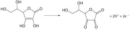
and for the analysis of reducing sugars, such as glucose, by oxidizing the aldehyde functional group to a carboxylate ion in a basic solution.
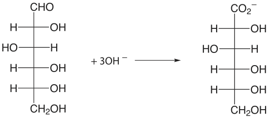
An organic compound that contains a hydroxyl, a carbonyl, or an amine functional group adjacent to an hydoxyl or a carbonyl group can be oxidized using metaperiodate, \(\text{IO}_4^-\), as an oxidizing titrant.
\[\text{IO}_4^-(aq) + \text{H}_2\text{O}(l) + 2e^- \rightleftharpoons \text{IO}_3^-(aq) + 2\text{OH}^-(aq) \nonumber\]
A two-electron oxidation cleaves the C–C bond between the two functional groups with hydroxyl groups oxidized to aldehydes or ketones, carbonyl groups oxidized to carboxylic acids, and amines oxidized to an aldehyde and an amine (ammonia if a primary amine). The analysis is conducted by adding a known excess of \(\text{IO}_4^-\) to the solution that contains the analyte and allowing the oxidation to take place for approximately one hour at room temperature. When the oxidation is complete, an excess of KI is added, which converts any unreacted \(\text{IO}_4^-\) to \(\text{IO}_3^-\) and \(\text{I}_3^-\).
\[\text{IO}_4^-(aq) + 3\text{I}^-(aq) + \text{H}_2\text{O}(l) \rightarrow \text{IO}_3^-(aq) + \text{I}_3^-(aq) + 2\text{OH}^-(aq) \nonumber\]
The \(\text{I}_3^-\) is then determined by titrating with \(\text{S}_2\text{O}_3^{2-}\) using starch as an indicator.
Quantitative Calculations
The quantitative relationship between the titrand and the titrant is determined by the stoichiometry of the titration reaction. If you are unsure of the balanced reaction, you can deduce its stoichiometry by remembering that the electrons in a redox reaction are conserved.
The amount of Fe in a 0.4891-g sample of an ore is determined by titrating with K2Cr2O7. After dissolving the sample in HCl, the iron is brought into a +2 oxidation state using a Jones reductor. Titration to the diphenylamine sulfonic acid end point requires 36.92 mL of 0.02153 M K2Cr2O7. Report the ore’s iron content as %w/w Fe2O3.
Solution
Because we are not provided with the titration reaction, we will use a conservation of electrons to deduce the stoichiometry. During the titration the analyte is oxidized from Fe2+ to Fe3+, and the titrant is reduced from \(\text{Cr}_2\text{O}_7^{2-}\) to Cr3+. Oxidizing Fe2+ to Fe3+ requires a single electron. Reducing \(\text{Cr}_2\text{O}_7^{2-}\), in which each chromium is in the +6 oxidation state, to Cr3+ requires three electrons per chromium, for a total of six electrons. A conservation of electrons for the titration, therefore, requires that each mole of K2Cr2O7 reacts with six moles of Fe2+.
The moles of K2Cr2O7 used to reach the end point is
\[(0.02153 \text{ M})(0.03692 \text{ L}) = 7.949 \times 10^{-4} \text{ mol K}_2\text{Cr}_2\text{O}_7 \nonumber\]
which means the sample contains
\[7.949 \times 10^{-4} \text{ mol K}_2\text{Cr}_2\text{O}_7 \times \frac{6 \text{ mol Fe}^{2+}}{\text{mol K}_2\text{Cr}_2\text{O}_7} = 4.769 \times 10^{-3} \text{ mol Fe}^{2+} \nonumber\]
Thus, the %w/w Fe2O3 in the sample of ore is
\[4.769 \times 10^{-3} \text{ mol Fe}^{2+} \times \frac{1 \text{ mol Fe}_2\text{O}_3}{2 \text{ mol Fe}^{2+}} \times \frac{159.69 \text{g Fe}_2\text{O}_3}{\text{mol Fe}_2\text{O}_3} = 0.3808 \text{ g Fe}_2\text{O}_3 \nonumber\]
\[\frac{0.3808 \text{ g Fe}_2\text{O}_3}{0.4891 \text{ g sample}} \times 100 = 77.86 \text{% w/w Fe}_2\text{O}_3 \nonumber\]
Although we can deduce the stoichiometry between the titrant and the titrand in Example 9.4.2 without balancing the titration reaction, the balanced reaction
\[\text{K}_2\text{Cr}_2\text{O}_7(aq) + 6\text{Fe}^{2+}(aq) + 14\text{H}^+(aq) \rightarrow 2\text{Cr}^{3+}(aq) + 2\text{K}^+(aq) + 6\text{Fe}^{3+}(aq) + 7\text{H}_2\text{O}(l) \nonumber\]
does provide useful information. For example, the presence of H+ reminds us that the reaction must take place in an acidic solution.
The purity of a sample of sodium oxalate, Na2C2O4, is determined by titrating with a standard solution of KMnO4. If a 0.5116-g sample requires 35.62 mL of 0.0400 M KMnO4 to reach the titration’s end point, what is the %w/w Na2C2O4 in the sample.
- Answer
-
Because we are not provided with a balanced reaction, let’s use a conservation of electrons to deduce the stoichiometry. Oxidizing \(\text{C}_2\text{O}_4^{2-}\), in which each carbon has a +3 oxidation state, to CO2, in which carbon has an oxidation state of +4, requires one electron per carbon or a total of two electrons for each mole of \(\text{C}_2\text{O}_4^{2-}\). Reducing \(\text{MnO}_4^-\), in which each manganese is in the +7 oxidation state, to Mn2+ requires five electrons. A conservation of electrons for the titration, therefore, requires that two moles of KMnO4 (10 moles of e-) react with five moles of Na2C2O4 (10 moles of e-).
The moles of KMnO4 used to reach the end point is
\[(0.0400 \text{ M KMnO}_4)(0.03562 \text{ L})=1.42 \times 10^{-3} \text{ mol KMnO}_4 \nonumber\]
which means the sample contains
\[1 .42 \times 10^{-3} \text{ mol KMnO}_4 \times \frac{5 \text{ mol Na}_2\text{C}_2\text{O}_4}{2 \text{ mol KMnO}_4} = 3.55 \times 10^{-3} \text{ mol Na}_2\text{C}_2\text{O}_4 \nonumber\]
Thus, the %w/w Na2C2O4 in the sample of ore is
\[3.55 \times 10^{-3} \text{ mol Na}_2\text{C}_2\text{O}_4 \times \frac{134.00 \text{ g Na}_2\text{C}_2\text{O}_4}{\text{mol Na}_2\text{C}_2\text{O}_4} = 0.476 \text{ g Na}_2\text{C}_2\text{O}_4 \nonumber\]
\[\frac{0.476 \text{ g Na}_2\text{C}_2\text{O}_4}{0.5116 \text{ g sample}} \times 100 = 93.0 \text{% w/w Na}_2\text{C}_2\text{O}_4 \nonumber\]
As shown in the following two examples, we can easily extend this approach to an analysis that requires an indirect analysis or a back titration.
A 25.00-mL sample of a liquid bleach is diluted to 1000 mL in a volumetric flask. A 25-mL portion of the diluted sample is transferred by pipet into an Erlenmeyer flask that contains an excess of KI, reducing the OCl– to Cl– and producing \(\text{I}_3^-\). The liberated \(\text{I}_3^-\) is determined by titrating with 0.09892 M Na2S2O3, requiring 8.96 mL to reach the starch indicator end point. Report the %w/v NaOCl in the sample of bleach.
Solution
To determine the stoichiometry between the analyte, NaOCl, and the titrant, Na2S2O3, we need to consider both the reaction between OCl– and I–, and the titration of \(\text{I}_3^-\) with Na2S2O3.
First, in reducing OCl– to Cl– the oxidation state of chlorine changes from +1 to –1, requiring two electrons. The oxidation of three I– to form \(\text{I}_3^-\) releases two electrons as the oxidation state of each iodine changes from –1 in I– to –1⁄3 in \(\text{I}_3^-\). A conservation of electrons, therefore, requires that each mole of OCl– produces one mole of \(\text{I}_3^-\).
Second, in the titration reaction, \(\text{I}_3^-\) is reduced to I– and \(\text{S}_2\text{O}_3^{2-}\) is oxidized to \(\text{S}_4\text{O}_6^{2-}\). Reducing \(\text{I}_3^-\) to 3I– requires two elections as each iodine changes from an oxidation state of –1⁄3 to –1. In oxidizing \(\text{S}_2\text{O}_3^{2-}\) to \(\text{S}_4\text{O}_6^{2-}\), each sulfur changes its oxidation state from +2 to +2.5, releasing one electron for each \(\text{S}_2\text{O}_3^{2-}\). A conservation of electrons, therefore, requires that each mole of \(\text{I}_3^-\) reacts with two moles of \(\text{S}_2\text{O}_3^{2-}\).
Finally, because each mole of OCl– produces one mole of \(\text{I}_3^-\), and each mole of \(\text{I}_3^-\) reacts with two moles of \(\text{S}_2\text{O}_3^{2-}\), we know that every mole of NaOCl in the sample ultimately results in the consumption of two moles of Na2S2O3.
The moles of Na2S2O3 used to reach the titration’s end point is
\[(0.09892 \text{ M})(0.00896 \text{ L}) = 8.86 \times 10^{-4} \text{ mol Na}_2\text{S}_2\text{O}_3 \nonumber\]
which means the sample contains
\[8.86 \times 10^{-4} \text{ mol Na}_2\text{S}_2\text{O}_3 \times \frac{1 \text{ mol NaOCl}}{\text{mol Na}_2\text{S}_2\text{O}_3} \times \frac{74.44 \text{ g NaOCl}}{\text{mol NaOCl}} = 0.03299 \text{ g NaOCl} \nonumber\]
Thus, the %w/v NaOCl in the diluted sample is
\[\frac{0.03299 \text{ g NaOCl}}{25.00 \text{ mL}} \times 100 = 0.132 \text{% w/v NaOCl} \nonumber\]
Because the bleach was diluted by a factor of \(40 \times\) (25 mL to 1000 mL), the concentration of NaOCl in the bleach is 5.28% w/v.
The balanced reactions for this analysis are:
\[\text{OCl}^-(aq) + 3\text{I}^-(aq) + 2\text{H}^+(aq) \rightarrow \text{I}_3^-(aq) + \text{Cl}^-(aq) + \text{H}_2\text{O}(l) \nonumber\]
\[\text{I}_3^-(aq) + 2\text{S}_2\text{O}_3^{2-}(aq) \rightarrow \text{S}_4\text{O}_6^{2-}(aq) + 3\text{I}^-(aq) \nonumber\]
The amount of ascorbic acid, C6H8O6, in orange juice is determined by oxidizing ascorbic acid to dehydroascorbic acid, C6H6O6, with a known amount of \(\text{I}_3^-\), and back titrating the excess \(\text{I}_3^-\) with Na2S2O3. A 5.00-mL sample of filtered orange juice is treated with 50.00 mL of 0.01023 M \(\text{I}_3^-\). After the oxidation is complete, 13.82 mL of 0.07203 M Na2S2O3 is needed to reach the starch indicator end point. Report the concentration ascorbic acid in mg/100 mL.
Solution
For a back titration we need to determine the stoichiometry between \(\text{I}_3^-\) and the analyte, C6H8O6, and between \(\text{I}_3^-\) and the titrant, Na2S2O3. The later is easy because we know from Example 9.4.3 that each mole of \(\text{I}_3^-\) reacts with two moles of Na2S2O3.
In oxidizing ascorbic acid to dehydroascorbic acid, the oxidation state of carbon changes from +2⁄3 in C6H8O6 to +1 in C6H6O6. Each carbon releases 1⁄3 of an electron, or a total of two electrons per ascorbic acid. As we learned in Example 9.4.3 , reducing \(\text{I}_3^-\) requires two electrons; thus, a conservation of electrons requires that each mole of ascorbic acid consumes one mole of \(\text{I}_3^-\).
The total moles of \(\text{I}_3^-\) that react with C6H8O6 and with Na2S2O3 is
\[(0.01023 \text{ M})(0.05000 \text{ L}) = 5.115 \times 10^{-4} \text{ mol I}_3^- \nonumber\]
The back titration consumes
\[0.01382 \text{ L Na}_2\text{S}_2\text{O}_3 \times \frac{0.07203 \text{ mol Na}_2\text{S}_2\text{O}_3}{\text{ L Na}_2\text{S}_2\text{O}_3} \times \frac{1 \text{ mol I}_3^-}{2 \text{ mol Na}_2\text{S}_2\text{O}_3} = 4.977 \times 10^{-4} \text{ mol I}_3^- \nonumber\]
Subtracting the moles of \(\text{I}_3^-\) that react with Na2S2O3 from the total moles of \(\text{I}_3^-\) gives the moles reacting with ascorbic acid.
\[5.115 \times 10^{-4} \text{ mol I}_3^- - 4.977 \times 10^{-4} \text{ mol I}_3^- = 1.38 \times 10^{-5} \text{ mol I}_3^- \nonumber\]
The grams of ascorbic acid in the 5.00-mL sample of orange juice is
\[1.38 \times 10^{-5} \text{ mol I}_3^- \times \frac{1 \text{ mol C}_6\text{H}_8\text{O}_6}{\text{mol I}_3^-} \times \frac{176.12 \text{ g C}_6\text{H}_8\text{O}_6}{\text{mol C}_6\text{H}_8\text{O}_6} = 2.43 \times 10^{-3} \text{ g C}_6\text{H}_8\text{O}_6 \nonumber\]
There are 2.43 mg of ascorbic acid in the 5.00-mL sample, or 48.6 mg per 100 mL of orange juice.
The balanced reactions for this analysis are:
\[\text{C}_6\text{H}_8\text{O}_6(aq) + \text{I}_3^- (aq) \rightarrow 3\text{I}^-(aq) + \text{C}_6\text{H}_6\text{O}_6(aq) + 2\text{H}^+(aq) \nonumber\]
\[\text{I}_3^-(aq) + 2\text{S}_2\text{O}_3^{2-}(aq) \rightarrow \text{S}_4\text{O}_6^{2-}(aq) + 3\text{I}^-(aq) \nonumber\]
A quantitative analysis for ethanol, C2H6O, is accomplished by a redox back titration. Ethanol is oxidized to acetic acid, C2H4O2, using excess dichromate, \(\text{Cr}_2\text{O}_7^{2-}\), which is reduced to Cr3+. The excess dichromate is titrated with Fe2+, giving Cr3+ and Fe3+ as products. In a typical analysis, a 5.00-mL sample of a brandy is diluted to 500 mL in a volumetric flask. A 10.00-mL sample is taken and the ethanol is removed by distillation and collected in 50.00 mL of an acidified solution of 0.0200 M K2Cr2O7. A back titration of the unreacted \(\text{Cr}_2\text{O}_7^{2-}\) requires 21.48 mL of 0.1014 M Fe2+. Calculate the %w/v ethanol in the brandy.
- Answer
-
For a back titration we need to determine the stoichiometry between \(\text{Cr}_2\text{O}_7^{2-}\) and the analyte, C2H6O, and between \(\text{Cr}_2\text{O}_7^{2-}\) and the titrant, Fe2+. In oxidizing ethanol to acetic acid, the oxidation state of carbon changes from –2 in C2H6O to 0 in C2H4O2. Each carbon releases two electrons, or a total of four electrons per C2H6O. In reducing \(\text{Cr}_2\text{O}_7^{2-}\), in which each chromium has an oxidation state of +6, to Cr3+, each chromium loses three electrons, for a total of six electrons per \(\text{Cr}_2\text{O}_7^{2-}\). Oxidation of Fe2+ to Fe3+ requires one electron. A conservation of electrons requires that each mole of K2Cr2O7 (6 moles of e–) reacts with six moles of Fe2+ (6 moles of e–), and that four moles of K2Cr2O7 (24 moles of e–) react with six moles of C2H6O (24 moles of e–).
The total moles of K2Cr2O7 that react with C2H6O and with Fe2+ is
\[(0.0200 \text{ M K}_2\text{Cr}_2\text{O}_7)(0.05000 \text{ L})=1.00 \times 10^{-3} \text{ mol K}_2\text{Cr}_2\text{O}_7 \nonumber\]
The back titration with Fe2+ consumes
\[(0.1014 \text{ M Fe}^{2+})(0.02148 \text{ L}) \times \frac{1 \text{ mol K}_2\text{Cr}_2\text{O}_7}{6 \text{ mol Fe}^{2+}} = 3.63 \times 10^{-4} \text{ mol K}_2\text{Cr}_2\text{O}_7 \nonumber\]
Subtracting the moles of K2Cr2O7 that react with Fe2+ from the total moles of K2Cr2O7 gives the moles that react with the analyte.
\[(1.00 \times 10^{-3} \text{ mol K}_2\text{Cr}_2\text{O}_7) - (3.63 \times 10^{-4} \text{ mol K}_2\text{Cr}_2\text{O}_7) = 6.37 \times 10^{-4} \text{ mol K}_2\text{Cr}_2\text{O}_7 \nonumber\]
The grams of ethanol in the 10.00-mL sample of diluted brandy is
\[6.37 \times 10^{-4} \text{ mol K}_2\text{Cr}_2\text{O}_7 \times \frac{6 \text{ mol C}_2\text{H}_6\text{O}}{4 \text{ mol K}_2\text{Cr}_2\text{O}_7} \times \frac{46.07 \text{ g C}_2\text{H}_6\text{O}}{\text{mol C}_2\text{H}_6\text{O}} = 0.0440 \text{ g C}_2\text{H}_6\text{O} \nonumber\]
The %w/v C2H6O in the brandy is
\[\frac{0.0440 \text{ g C}_2\text{H}_6\text{O}}{10.0 \text{ mL diluted brandy}} \times \frac{500.0 \text{ mL diluted brandy}}{5.00 \text{ mL brandy}} \times 100 = 44.0 \text{% w/v C}_2\text{H}_6\text{O} \nonumber\]
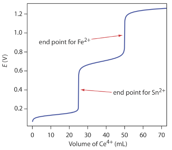
Evaluation of Redox Titrimetry
The scale of operations, accuracy, precision, sensitivity, time, and cost of a redox titration are similar to those described earlier in this chapter for an acid–base or a complexation titration. As with an acid–base titration, we can extend a redox titration to the analysis of a mixture of analytes if there is a significant difference in their oxidation or reduction potentials. Figure 9.4.7 shows an example of the titration curve for a mixture of Fe2+ and Sn2+ using Ce4+ as the titrant. A titration of a mixture of analytes is possible if their standard state potentials or formal potentials differ by at least 200 mV.