Search

Text Color

Margin Size

Font Type

Enable Dyslexic Font

2.3: First-Order Reactions

Last updated

Feb 13, 2023
Save as PDF
- 2.2: Factors That Affect Reaction Rates
- 2.4: Half-lives

$\newcommand{\vecs}[1]{\overset { \scriptstyle \rightharpoonup} {\mathbf{#1}} }$

$\newcommand{\vecd}[1]{\overset{-\!-\!\rightharpoonup}{\vphantom{a}\smash {#1}}}$

$\newcommand{\id}{\mathrm{id}}$ $\newcommand{\Span}{\mathrm{span}}$

( \newcommand{\kernel}{\mathrm{null}\,}\) $\newcommand{\range}{\mathrm{range}\,}$

$\newcommand{\RealPart}{\mathrm{Re}}$ $\newcommand{\ImaginaryPart}{\mathrm{Im}}$

$\newcommand{\Argument}{\mathrm{Arg}}$ $\newcommand{\norm}[1]{\| #1 \|}$

$\newcommand{\inner}[2]{\langle #1, #2 \rangle}$

$\newcommand{\Span}{\mathrm{span}}$

$\newcommand{\id}{\mathrm{id}}$

$\newcommand{\Span}{\mathrm{span}}$

$\newcommand{\kernel}{\mathrm{null}\,}$

$\newcommand{\range}{\mathrm{range}\,}$

$\newcommand{\RealPart}{\mathrm{Re}}$

$\newcommand{\ImaginaryPart}{\mathrm{Im}}$

$\newcommand{\Argument}{\mathrm{Arg}}$

$\newcommand{\norm}[1]{\| #1 \|}$

$\newcommand{\inner}[2]{\langle #1, #2 \rangle}$

$\newcommand{\Span}{\mathrm{span}}$ $\newcommand{\AA}{\unicode[.8,0]{x212B}}$

$\newcommand{\vectorA}[1]{\vec{#1}} % arrow$

$\newcommand{\vectorAt}[1]{\vec{\text{#1}}} % arrow$

$\newcommand{\vectorB}[1]{\overset { \scriptstyle \rightharpoonup} {\mathbf{#1}} }$

$\newcommand{\vectorC}[1]{\textbf{#1}}$

$\newcommand{\vectorD}[1]{\overrightarrow{#1}}$

$\newcommand{\vectorDt}[1]{\overrightarrow{\text{#1}}}$

$\newcommand{\vectE}[1]{\overset{-\!-\!\rightharpoonup}{\vphantom{a}\smash{\mathbf {#1}}}}$

$\newcommand{\vecs}[1]{\overset { \scriptstyle \rightharpoonup} {\mathbf{#1}} }$

$\newcommand{\vecd}[1]{\overset{-\!-\!\rightharpoonup}{\vphantom{a}\smash {#1}}}$

$\newcommand{\avec}{\mathbf a}$

$\newcommand{\bvec}{\mathbf b}$

$\newcommand{\cvec}{\mathbf c}$

$\newcommand{\dvec}{\mathbf d}$

$\newcommand{\dtil}{\widetilde{\mathbf d}}$

$\newcommand{\evec}{\mathbf e}$

$\newcommand{\fvec}{\mathbf f}$

$\newcommand{\nvec}{\mathbf n}$

$\newcommand{\pvec}{\mathbf p}$

$\newcommand{\qvec}{\mathbf q}$

$\newcommand{\svec}{\mathbf s}$

$\newcommand{\tvec}{\mathbf t}$

$\newcommand{\uvec}{\mathbf u}$

$\newcommand{\vvec}{\mathbf v}$

$\newcommand{\wvec}{\mathbf w}$

$\newcommand{\xvec}{\mathbf x}$

$\newcommand{\yvec}{\mathbf y}$

$\newcommand{\zvec}{\mathbf z}$

$\newcommand{\rvec}{\mathbf r}$

$\newcommand{\mvec}{\mathbf m}$

$\newcommand{\zerovec}{\mathbf 0}$

$\newcommand{\onevec}{\mathbf 1}$

$\newcommand{\real}{\mathbb R}$

$\newcommand{\twovec}[2]{\left[\begin{array}{r}#1 \\ #2 \end{array}\right]}$

$\newcommand{\ctwovec}[2]{\left[\begin{array}{c}#1 \\ #2 \end{array}\right]}$

$\newcommand{\threevec}[3]{\left[\begin{array}{r}#1 \\ #2 \\ #3 \end{array}\right]}$

$\newcommand{\cthreevec}[3]{\left[\begin{array}{c}#1 \\ #2 \\ #3 \end{array}\right]}$

$\newcommand{\fourvec}[4]{\left[\begin{array}{r}#1 \\ #2 \\ #3 \\ #4 \end{array}\right]}$

$\newcommand{\cfourvec}[4]{\left[\begin{array}{c}#1 \\ #2 \\ #3 \\ #4 \end{array}\right]}$

$\newcommand{\fivevec}[5]{\left[\begin{array}{r}#1 \\ #2 \\ #3 \\ #4 \\ #5 \\ \end{array}\right]}$

$\newcommand{\cfivevec}[5]{\left[\begin{array}{c}#1 \\ #2 \\ #3 \\ #4 \\ #5 \\ \end{array}\right]}$

$\newcommand{\mattwo}[4]{\left[\begin{array}{rr}#1 \amp #2 \\ #3 \amp #4 \\ \end{array}\right]}$

$\newcommand{\laspan}[1]{\text{Span}\{#1\}}$

$\newcommand{\bcal}{\cal B}$

$\newcommand{\ccal}{\cal C}$

$\newcommand{\scal}{\cal S}$

$\newcommand{\wcal}{\cal W}$

$\newcommand{\ecal}{\cal E}$

$\newcommand{\coords}[2]{\left\{#1\right\}_{#2}}$

$\newcommand{\gray}[1]{\color{gray}{#1}}$

$\newcommand{\lgray}[1]{\color{lightgray}{#1}}$

$\newcommand{\rank}{\operatorname{rank}}$

$\newcommand{\row}{\text{Row}}$

$\newcommand{\col}{\text{Col}}$

$\renewcommand{\row}{\text{Row}}$

$\newcommand{\nul}{\text{Nul}}$

$\newcommand{\var}{\text{Var}}$

$\newcommand{\corr}{\text{corr}}$

$\newcommand{\len}[1]{\left|#1\right|}$

$\newcommand{\bbar}{\overline{\bvec}}$

$\newcommand{\bhat}{\widehat{\bvec}}$

$\newcommand{\bperp}{\bvec^\perp}$

$\newcommand{\xhat}{\widehat{\xvec}}$

$\newcommand{\vhat}{\widehat{\vvec}}$

$\newcommand{\uhat}{\widehat{\uvec}}$

$\newcommand{\what}{\widehat{\wvec}}$

$\newcommand{\Sighat}{\widehat{\Sigma}}$

$\newcommand{\lt}{<}$

$\newcommand{\gt}{>}$

$\newcommand{\amp}{&}$

$\definecolor{fillinmathshade}{gray}{0.9}$

A first-order reaction is a reaction that proceeds at a rate that depends linearly on only one reactant concentration.

The Differential Representation

Differential rate laws are generally used to describe what is occurring on a molecular level during a reaction, whereas integrated rate laws are used for determining the reaction order and the value of the rate constant from experimental measurements. The differential equation describing first-order kinetics is given below:

$Rate = - \dfrac{d[A]}{dt} = k[A]^1 = k[A] \label{1}$

is the reaction rate (in units of molar/time) and $k$ is the reaction rate coefficient (in units of 1/time). However, the units of $k$ vary for non-first-order reactions. These differential equations are separable, which simplifies the solutions as demonstrated below.

The Integral Representation

First, write the differential form of the rate law.

$Rate = - \dfrac{d[A]}{dt} = k[A] \nonumber$

Rearrange to give:

$\dfrac{d[A]}{[A]} = - k\,dt \nonumber$

Second, integrate both sides of the equation.

$\begin{align*} \int_{[A]_o}^{[A]} \dfrac{d[A]}{[A]} &= -\int_{t_o}^{t} k\, dt \label{4a} \\[4pt] \int_{[A]_{o}}^{[A]} \dfrac{1}{[A]} d[A] &= -\int_{t_o}^{t} k\, dt \label{4b} \end{align*}$

Recall from calculus that:

$\int \dfrac{1}{x} = \ln(x) \nonumber$

Upon integration,

$\ln[A] - \ln[A]_o = -kt \nonumber$

Rearrange to solve for [A] to obtain one form of the rate law:

$\ln[A] = \ln[A]_o - kt \nonumber$

This can be rearranged to:

$\ln [A] = -kt + \ln [A]_o \nonumber$

This can further be arranged into y=mx +b form:

$\ln [A] = -kt + \ln [A]_o \nonumber$

The equation is a straight line with slope m:

$mx=-kt \nonumber$

and y-intercept b:

$b=\ln [A]_o \nonumber$

Now, recall from the laws of logarithms that

$\ln {\left(\dfrac{[A]_t}{ [A]_o}\right)}= -kt \nonumber$

where [A] is the concentration at time $t$ and $[A]_o$ is the concentration at time 0, and $k$ is the first-order rate constant.

Figure $\PageIndex{1}$ : Decay profiles for first-order reactions with large and small rate constants. (CC BY; Stephen Lower)

Because the logarithms of numbers do not have any units, the product $-kt$ also lacks units. This concludes that unit of $k$ in a first order of reaction must be time^-1. Examples of time^-1include s^-1 or min^-1. Thus, the equation of a straight line is applicable:

$\ln [A] = -kt + \ln [A]_o.\label{15}$

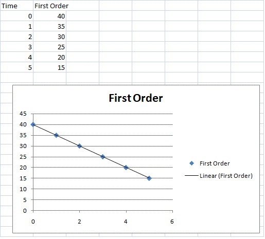
To test if it the reaction is a first-order reaction, plot the natural logarithm of a reactant concentration versus time and see whether the graph is linear. If the graph is linear and has a negative slope, the reaction must be a first-order reaction.

To create another form of the rate law, raise each side of the previous equation to the exponent, $e$ :

$\large e^{\ln[A]} = e^{\ln[A]_o - kt} \label{16}$

Simplifying gives the second form of the rate law:

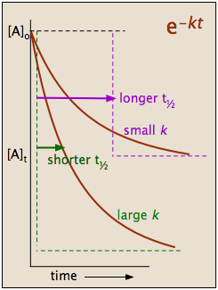
$[A] = [A]_{o}e^{- kt}\label{17}$

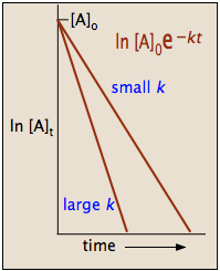
The integrated forms of the rate law can be used to find the population of reactant at any time after the start of the reaction. Plotting $\ln[A]$ with respect to time for a first-order reaction gives a straight line with the slope of the line equal to $-k$ . More information can be found in the article on rate laws.

This general relationship, in which a quantity changes at a rate that depends on its instantaneous value, is said to follow an exponential law. Exponential relations are widespread in science and in many other fields. Consumption of a chemical reactant or the decay of a radioactive isotope follow the exponential decay law. Its inverse, the law of exponential growth, describes the manner in which the money in a continuously-compounding bank account grows with time, or the population growth of a colony of reproducing organisms. The reason that the exponential function $y=e^x$ so efficiently describes such changes is that dy/dx = e^x; that is, e^x is its own derivative, making the rate of change of $y$ identical to its value at any point.

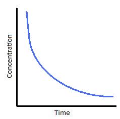
Graphing First-order Reactions

The following graphs represents concentration of reactants versus time for a first-order reaction.

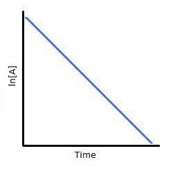
Plotting $\ln[A]$ with respect to time for a first-order reaction gives a straight line with the slope of the line equal to $-k$ .

First order.jpg

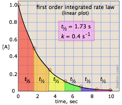
Half-lives of first order reactions

The half-life ( $t_{1/2}$ ) is a timescale on which the initial population is decreased by half of its original value, represented by the following equation.

$[A] = \dfrac{1}{2} [A]_o \nonumber$

After a period of one half-life, $t = t_{1/2}$ and we can write

$\dfrac{[A]_{1/2}}{[A]_o} = \dfrac{1}{2}=e^{-k\,t_{1/2}} \label{18}$

Taking logarithms of both sides (remember that $\ln e^x = x$ ) yields

$\ln 0.5 = -kt\label{19}$

Solving for the half-life, we obtain the simple relation

$t_{1/2}=\dfrac{\ln{2}}{k} \approx \dfrac{0.693}{k}\label{20}$

This indicates that the half-life of a first-order reaction is a constant.

Figure $\PageIndex{2}$ : Half lives graphically demonstrated for first-order reaction. Notice the the half-life is independent of initial concentration. This is not the case with other reaction orders. (CC BY; Stephen Lower)

Example 1: Estimated Rate Constants

The half-life of a first-order reaction was found to be 10 min at a certain temperature. What is its rate constant?

Solution

Use Equation 20 that relates half life to rate constant for first order reactions:

$k = \dfrac{0.693}{600 \;s} = 0.00115 \;s^{-1} \nonumber$

As a check, dimensional analysis can be used to confirm that this calculation generates the correct units of inverse time.

Notice that, for first-order reactions, the half-life is independent of the initial concentration of reactant, which is a unique aspect to first-order reactions. The practical implication of this is that it takes as much time for [A] to decrease from 1 M to 0.5 M as it takes for [A] to decrease from 0.1 M to 0.05 M. In addition, the rate constant and the half life of a first-order process are inversely related.

Example $\PageIndex{1}$ : Determining Half life

If 3.0 g of substance $A$ decomposes for 36 minutes the mass of unreacted A remaining is found to be 0.375 g. What is the half life of this reaction if it follows first-order kinetics?

Solution

There are two ways to approach this problem: The "simple inspection approach" and the "brute force approach"

Approach #1: "The simple Inspection Approach"

This approach is used when one can recognize that the final concentration of $A$ is $\frac{1}{8}$ of the initial concentration and hence three half lives $\left(\frac{1}{2} \times \frac{1}{2} \times \frac{1}{2}\right)$ have elapsed during this reaction.

$t_{1/2} = \dfrac{36\, \text{min}}{3}= 12 \; \text{min} \nonumber$

This approach works only when the final concentration is $\left(\frac{1}{2}\right)^n$ that of the initial concentration, then $n$ is the number of half lives that have elapsed. If this is not the case, then approach #2 can be used.

Approach #2: "The brute force approach"

e $t_{1/2}$ $\begin{align*} \dfrac{[A]_t}{[A]_o} &= e^{-k\,t} \\[4pt] k &= -\dfrac{\ln \dfrac{[A]_t}{[A]_o}}{t} \\[4pt] &= -\dfrac{\ln \dfrac{0.375\, g}{3\, g}}{36\, \text{min}} \\[4pt] &= 0.0578 \, \text{min}^{-1} \end{align*}$ Therefore, via Equation $\ref{20}$ $t_{1/2}=\dfrac{\ln{2}}{k} \approx \dfrac{0.693}{0.0578 \, \text{min}^{-1}} \approx 12\, \text{min} \nonumber$

The first approach is considerably faster (if the number of half lives evolved is apparent).

Exercise $\PageIndex{2a}$

Calculate the half-life of the reactions below:

If 4.00 g A are allowed to decompose for 40 min, the mass of A remaining undecomposed is found to be 0.80 g.
If 8.00 g A are allowed to decompose for 34 min, the mass of A remaining undecomposed is found to be 0.70 g.
If 9.00 g A are allowed to decompose for 24 min, the mass of A remaining undecomposed is found to be 0.50 g.

Answer

Use the half life reaction that contains initial concentration and final concentration. Plug in the appropriate variables and solve to obtain:

17.2 min
9.67 min
5.75 min

Exercise $\PageIndex{2b}$

Determine the percent $\ce{H2O2}$ that decomposes in the time using $k=6.40 \times 10^{-5} s^{-1}$

The time for the concentration to decompose is 600.0 s after the reaction begins.
The time for the concentration to decompose is 450 s after the reaction begins.

Answer

Rearranging Eq. 17 to solve for the $[H_2O_2]_t/[H_2O_2]_0$ ratio $\dfrac{[H_2O_2]_t}{[H_2O_2]_0} = e^{-kt} \nonumber$ This is a simple plug and play application once you have identified this equation. $\dfrac{[H_2O_2]_{t=600\;s}}{[H_2O_2]_0} = e^{-(6.40 \times 10^{-5} s^{-1}) (600 \, s)} \nonumber$ $\dfrac{[H_2O_2]_{t=600\;s}}{[H_2O_2]_0} = 0.9629 \nonumber$ So 100-96.3=3.71% of the hydrogen peroxide has decayed by 600 s.
Rearranging Eq. 17 to solve for the $[H_2O_2]_t/[H_2O_2]_0$ ratio $\dfrac{[H_2O_2]_t}{[H_2O_2]_0} = e^{-kt} \nonumber$ This is a simple plug and play application once you have identified this equation. $\dfrac{[H_2O_2]_{t=450\;s}}{[H_2O_2]_0} = e^{-(6.40 \times 10^{-5} s^{-1}) (450 \, s)} \nonumber$ $\dfrac{[H_2O_2]_{t=450\;s}}{[H_2O_2]_0} = 0.9720 \nonumber$ So 100-97.2=2.8% of the hydrogen peroxide has decayed by 450 s.

References

Petrucci, Ralph H. General Chemistry: Principles and Modern Applications 9th Ed. New Jersey: Pearson Education Inc. 2007.

Contributors and Attributions

Rachael Curtis (UCD), Cathy Nguyen (UCD)
Stephen Lower, Professor Emeritus (Simon Fraser U.) Chem1 Virtual Textbook

The Differential Representation

The Integral Representation

Graphing First-order Reactions

Half-lives of first order reactions

Example 1: Estimated Rate Constants

Example \PageIndex{1}\PageIndex{1}: Determining Half life

Solution

Exercise \PageIndex{2a}\PageIndex{2a}

Exercise \PageIndex{2b}\PageIndex{2b}

References

Contributors and Attributions

Support Center

How can we help?

Example $\PageIndex{1}$ : Determining Half life

Exercise $\PageIndex{2a}$

Exercise $\PageIndex{2b}$