2.4: Half-lives
- Page ID
- 1434
\( \newcommand{\vecs}[1]{\overset { \scriptstyle \rightharpoonup} {\mathbf{#1}} } \)
\( \newcommand{\vecd}[1]{\overset{-\!-\!\rightharpoonup}{\vphantom{a}\smash {#1}}} \)
\( \newcommand{\id}{\mathrm{id}}\) \( \newcommand{\Span}{\mathrm{span}}\)
( \newcommand{\kernel}{\mathrm{null}\,}\) \( \newcommand{\range}{\mathrm{range}\,}\)
\( \newcommand{\RealPart}{\mathrm{Re}}\) \( \newcommand{\ImaginaryPart}{\mathrm{Im}}\)
\( \newcommand{\Argument}{\mathrm{Arg}}\) \( \newcommand{\norm}[1]{\| #1 \|}\)
\( \newcommand{\inner}[2]{\langle #1, #2 \rangle}\)
\( \newcommand{\Span}{\mathrm{span}}\)
\( \newcommand{\id}{\mathrm{id}}\)
\( \newcommand{\Span}{\mathrm{span}}\)
\( \newcommand{\kernel}{\mathrm{null}\,}\)
\( \newcommand{\range}{\mathrm{range}\,}\)
\( \newcommand{\RealPart}{\mathrm{Re}}\)
\( \newcommand{\ImaginaryPart}{\mathrm{Im}}\)
\( \newcommand{\Argument}{\mathrm{Arg}}\)
\( \newcommand{\norm}[1]{\| #1 \|}\)
\( \newcommand{\inner}[2]{\langle #1, #2 \rangle}\)
\( \newcommand{\Span}{\mathrm{span}}\) \( \newcommand{\AA}{\unicode[.8,0]{x212B}}\)
\( \newcommand{\vectorA}[1]{\vec{#1}} % arrow\)
\( \newcommand{\vectorAt}[1]{\vec{\text{#1}}} % arrow\)
\( \newcommand{\vectorB}[1]{\overset { \scriptstyle \rightharpoonup} {\mathbf{#1}} } \)
\( \newcommand{\vectorC}[1]{\textbf{#1}} \)
\( \newcommand{\vectorD}[1]{\overrightarrow{#1}} \)
\( \newcommand{\vectorDt}[1]{\overrightarrow{\text{#1}}} \)
\( \newcommand{\vectE}[1]{\overset{-\!-\!\rightharpoonup}{\vphantom{a}\smash{\mathbf {#1}}}} \)
\( \newcommand{\vecs}[1]{\overset { \scriptstyle \rightharpoonup} {\mathbf{#1}} } \)
\( \newcommand{\vecd}[1]{\overset{-\!-\!\rightharpoonup}{\vphantom{a}\smash {#1}}} \)
\(\newcommand{\avec}{\mathbf a}\) \(\newcommand{\bvec}{\mathbf b}\) \(\newcommand{\cvec}{\mathbf c}\) \(\newcommand{\dvec}{\mathbf d}\) \(\newcommand{\dtil}{\widetilde{\mathbf d}}\) \(\newcommand{\evec}{\mathbf e}\) \(\newcommand{\fvec}{\mathbf f}\) \(\newcommand{\nvec}{\mathbf n}\) \(\newcommand{\pvec}{\mathbf p}\) \(\newcommand{\qvec}{\mathbf q}\) \(\newcommand{\svec}{\mathbf s}\) \(\newcommand{\tvec}{\mathbf t}\) \(\newcommand{\uvec}{\mathbf u}\) \(\newcommand{\vvec}{\mathbf v}\) \(\newcommand{\wvec}{\mathbf w}\) \(\newcommand{\xvec}{\mathbf x}\) \(\newcommand{\yvec}{\mathbf y}\) \(\newcommand{\zvec}{\mathbf z}\) \(\newcommand{\rvec}{\mathbf r}\) \(\newcommand{\mvec}{\mathbf m}\) \(\newcommand{\zerovec}{\mathbf 0}\) \(\newcommand{\onevec}{\mathbf 1}\) \(\newcommand{\real}{\mathbb R}\) \(\newcommand{\twovec}[2]{\left[\begin{array}{r}#1 \\ #2 \end{array}\right]}\) \(\newcommand{\ctwovec}[2]{\left[\begin{array}{c}#1 \\ #2 \end{array}\right]}\) \(\newcommand{\threevec}[3]{\left[\begin{array}{r}#1 \\ #2 \\ #3 \end{array}\right]}\) \(\newcommand{\cthreevec}[3]{\left[\begin{array}{c}#1 \\ #2 \\ #3 \end{array}\right]}\) \(\newcommand{\fourvec}[4]{\left[\begin{array}{r}#1 \\ #2 \\ #3 \\ #4 \end{array}\right]}\) \(\newcommand{\cfourvec}[4]{\left[\begin{array}{c}#1 \\ #2 \\ #3 \\ #4 \end{array}\right]}\) \(\newcommand{\fivevec}[5]{\left[\begin{array}{r}#1 \\ #2 \\ #3 \\ #4 \\ #5 \\ \end{array}\right]}\) \(\newcommand{\cfivevec}[5]{\left[\begin{array}{c}#1 \\ #2 \\ #3 \\ #4 \\ #5 \\ \end{array}\right]}\) \(\newcommand{\mattwo}[4]{\left[\begin{array}{rr}#1 \amp #2 \\ #3 \amp #4 \\ \end{array}\right]}\) \(\newcommand{\laspan}[1]{\text{Span}\{#1\}}\) \(\newcommand{\bcal}{\cal B}\) \(\newcommand{\ccal}{\cal C}\) \(\newcommand{\scal}{\cal S}\) \(\newcommand{\wcal}{\cal W}\) \(\newcommand{\ecal}{\cal E}\) \(\newcommand{\coords}[2]{\left\{#1\right\}_{#2}}\) \(\newcommand{\gray}[1]{\color{gray}{#1}}\) \(\newcommand{\lgray}[1]{\color{lightgray}{#1}}\) \(\newcommand{\rank}{\operatorname{rank}}\) \(\newcommand{\row}{\text{Row}}\) \(\newcommand{\col}{\text{Col}}\) \(\renewcommand{\row}{\text{Row}}\) \(\newcommand{\nul}{\text{Nul}}\) \(\newcommand{\var}{\text{Var}}\) \(\newcommand{\corr}{\text{corr}}\) \(\newcommand{\len}[1]{\left|#1\right|}\) \(\newcommand{\bbar}{\overline{\bvec}}\) \(\newcommand{\bhat}{\widehat{\bvec}}\) \(\newcommand{\bperp}{\bvec^\perp}\) \(\newcommand{\xhat}{\widehat{\xvec}}\) \(\newcommand{\vhat}{\widehat{\vvec}}\) \(\newcommand{\uhat}{\widehat{\uvec}}\) \(\newcommand{\what}{\widehat{\wvec}}\) \(\newcommand{\Sighat}{\widehat{\Sigma}}\) \(\newcommand{\lt}{<}\) \(\newcommand{\gt}{>}\) \(\newcommand{\amp}{&}\) \(\definecolor{fillinmathshade}{gray}{0.9}\)The half-life of a reaction (\(t_{1/2}\)), is the amount of time needed for a reactant concentration to decrease by half compared to its initial concentration. Its application is used in chemistry and medicine to predict the concentration of a substance over time. The concepts of half life plays a key role in the administration of drugs into the target, especially in the elimination phase, where half life is used to determine how quickly a drug decrease in the target after it has been absorbed in units of time (e.g., s, min., day, etc.) or elimination rate constant \(k\) in units of 1/time (e.g., min-1, hr-1, day-1, etc.). It is important to note that the half-life is varied between different type of reactions. The following section will go over different type of reaction, as well as how its half-life reaction are derived. The last section will talk about the application of half-life in the elimination phase of pharmacokinetics.
Zero-Order Kinetics
In zero-order kinetics, the rate of a reaction does not depend on the substrate concentration. In other words, saturating the amount of substrate does not speed up the rate of the reaction. Below is a graph of time (\(t\)) vs. concentration (\([A]\)) in a zero order reaction, several observation can be made: the slope of this plot is a straight line with negative slope equal negative \(k\), the half-life of zero order reaction decreases as the concentration decreases.
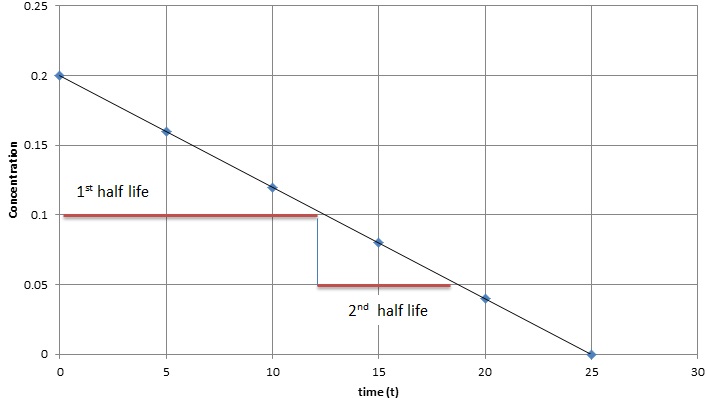
We learn that the zero-order kinetic rate law is as followed, where \([A]\) is the current concentration, \([A]_o\) is the initial concentration, and \(k\) is the reaction constant and \(t\) is time:
\[ [A]= [A]_o - kt \label{1} \]
We need to isolate \(t_{1/2}\) when
\[[A]=\dfrac{[A]_o}{2} \nonumber \]
Substituting into Equation \ref{1}
\[\begin{align} \dfrac{[A]_o}{2} &= [A]_o - kt_{1/2} \nonumber \\[4pt] kt_{1/2} &= [A]_o - \dfrac{[A]_o}{2} \nonumber \\[4pt] t_{1/2} &= \dfrac{[A]_o}{2k} \label{2} \end{align} \]
Equation \ref{2} show the half-life for a zero-order reaction depends on both the initial concentration and rate constant.
First-Order Kinetics
In First order reactions, the graph represents the half-life is different from zero order reaction in a way that the slope continually decreases as time progresses until it reaches zero. We can also easily see that the length of half-life will be constant, independent of concentration. For example, it takes the same amount of time for the concentration to decrease from one point to another point.
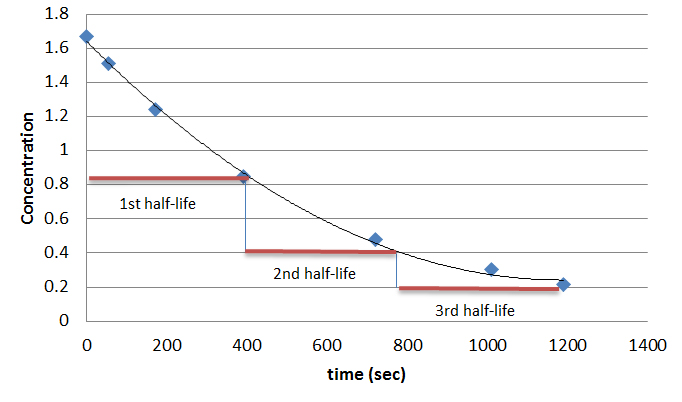
In order to solve the half life of first order reactions, we recall that the rate law of a first order reaction was:
\[[A]=[A]_o e^{-kt} \label{4} \]
We need to isolate \(t_{1/2}\) when
\[[A]=\dfrac{[A]_o}{2} \nonumber \]
Substituting into Equation \ref{4}
\[ \begin{align} \dfrac{[A]_0}{2} &=[A]_o e^{-kt_{1/2}} \nonumber \\[4pt] \dfrac{1}{2} &= e^{-kt_{1/2}} \nonumber \\[4pt] \ln \dfrac{1}{2} &= -kt_{1/2} \nonumber \\[4pt] t_{1/2} &= \dfrac{\ln 2}{k} \nonumber \\[4pt] &\approx \dfrac{0.693}{k} \label{5} \end{align} \]
Equation \ref{5} shows that for first-order reactions, the half-life depends solely on the reaction rate constant, \(k\). We can visually see this on the graph for first order reactions when we note that the amount of time between one half life and the next are the same. Another way to see it is that the half life of a first order reaction is independent of its initial concentration.
Second-Order Kinetics
Half-life of second order reactions shows concentration \([A]\) vs. time (\(t\)), which is similar to first order plots in that their slopes decrease to zero with time. However, second order reactions decrease at a much faster rate as the graph shows. We can also note that the length of half-life increase while the concentration of substrate constantly decreases, unlike zero and first order reaction.
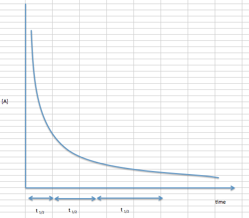
In order to solve for half life of second order reactions we need to remember that the rate law of a second order reaction is:
\[\dfrac{1}{[A]} = kt + \dfrac{1}{[A]_0} \label{6} \]
As in zero-order and first-order reactions, we need to isolate \(t_{1/2}\) when
\[[A]=\dfrac{[A]_o}{2} \nonumber \]
Substituting into Equation \ref{6}
\[ \begin{align} \dfrac{2}{[A]_0} &= kt_{1/2} + \dfrac{1}{[A]_0}\nonumber \\[4pt] -kt_{1/2} &= \dfrac{1}{[A]_0} - \dfrac{2}{[A]_0} \nonumber \\[4pt] t_{1/2} &= \dfrac{1}{k[A]_0} \label{7} \end{align} \]
Equation \ref{7} shows that for second-order reactions, the half-life depends on both the initial concentration and the rate constant.
A following example is given below to illustrate the role of half life in pharmacokinetics to determine the drugs dosage interval.
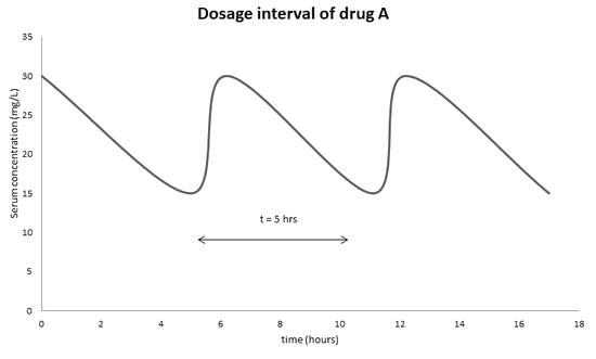
The therapeutic range of drug A is 15-30 mg/L. Its half life in the target in 5 hours. Once the drug is metabolized in the target, its concentration will decrease over time. To ensure its maximal effect of the drug in the target, the administration will be monitored so that the minimum serum concentration will never go lower than 15 mg/L and the maximum serum concentration will never exceed 30 mg/L. As a result, it is important to administer drug A to the target every 5 hours to ensure its effective therapeutic range.
Another important application of half life in pharmacokinetics is that half-life tells how tightly drugs bind to each ligands before it is undergoing decay (\(k_s\)). The smaller the value of \(k_s\), the higher the affinity binding of drug to its target ligand, which is an important aspect of drug design
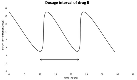
Examine the following graph and answer
- What is the therapeutic range of drug B?
- From the graph, estimate the dosage interval of drug B to ensure its maximum effect?
- The patient forgot to take the drug at the end of the dosage interval, he decided to take double the amount of drug B at the end of the next dosage interval. Will the drug still be in its therapeutic range?
- Answer
-
Looking at the graph, we can see the therapeutic range is the amplitude of the graph, which is 5-15 mg/L
The dosage interval is the half-life of the drug, looking at the graph, the half-life is 10 hours.
Even though it will get in the therapeutic range, such practice is not recommended.
A patient is treating with \(\ce{^{32}P}\). How long does it takes for the radioactivity to decay by 90%? The half-life of the material is 15 days.
- Answer
-
If we want the product to decay by 90%, that means 10% is left non-decayed, so
\[\dfrac{[A]_t}{[A]_o} = 0.1 \nonumber \]
From ln([A]t/[A]o) = -kt, plug in value of k and [A]t/[A]o we then have t = 50 days
In first order half life, what is the best way to determine the rate constant \(k\)? Why?
- Answer
-
The best way to determine rate constant \(k\) in half-life of first order is to determine half-life by experimental data. The reason is half-life in first order order doesn't depend on initial concentration.
In a first order reaction, \(\ce{A -> B}\). The half-life is 10 days.
- Determine its rate constant \(k\)?
- How much time required for this reaction to be at least 50% and 60% complete?
- Answer
-
- This is a direct application of Equation \ref{7}. The rate constant, \(k\), will be equal to \[k=\dfrac{\ln 2}{t_{1/2}} \nonumber \] so \(k = 0.0693 \,day^{-1}\).
- For the reaction to be 50% complete, that will be exactly the half-life of the reaction at 10 days. For the reaction to be 60% complete, using the similar equation derived from question 4, we have \[\dfrac{[A]_t}{[A]_o} = 0.4 \nonumber \] \[t = 13.2\, days \nonumber \]
References
- Chang, Raymond. Physical Chemistry for the Biosciences. Sausalito,CA: University Science Books. Pages 312-319. 2005
- Bauer, Larry. Applied Clinical Pharmacokinetics. New York City, New York: McGraw-Hill. 2008
- Mozayani, Ashraf and Raymond, Lionel. Handbook of Drug Interactions: A Clinical and Forensic Guide. Totowa, New Jersy: Humana Press. 2003


