
2.8: Second-Order Reactions
- Page ID
- 1440
\( \newcommand{\vecs}[1]{\overset { \scriptstyle \rightharpoonup} {\mathbf{#1}} } \)
\( \newcommand{\vecd}[1]{\overset{-\!-\!\rightharpoonup}{\vphantom{a}\smash {#1}}} \)
\( \newcommand{\id}{\mathrm{id}}\) \( \newcommand{\Span}{\mathrm{span}}\)
( \newcommand{\kernel}{\mathrm{null}\,}\) \( \newcommand{\range}{\mathrm{range}\,}\)
\( \newcommand{\RealPart}{\mathrm{Re}}\) \( \newcommand{\ImaginaryPart}{\mathrm{Im}}\)
\( \newcommand{\Argument}{\mathrm{Arg}}\) \( \newcommand{\norm}[1]{\| #1 \|}\)
\( \newcommand{\inner}[2]{\langle #1, #2 \rangle}\)
\( \newcommand{\Span}{\mathrm{span}}\)
\( \newcommand{\id}{\mathrm{id}}\)
\( \newcommand{\Span}{\mathrm{span}}\)
\( \newcommand{\kernel}{\mathrm{null}\,}\)
\( \newcommand{\range}{\mathrm{range}\,}\)
\( \newcommand{\RealPart}{\mathrm{Re}}\)
\( \newcommand{\ImaginaryPart}{\mathrm{Im}}\)
\( \newcommand{\Argument}{\mathrm{Arg}}\)
\( \newcommand{\norm}[1]{\| #1 \|}\)
\( \newcommand{\inner}[2]{\langle #1, #2 \rangle}\)
\( \newcommand{\Span}{\mathrm{span}}\) \( \newcommand{\AA}{\unicode[.8,0]{x212B}}\)
\( \newcommand{\vectorA}[1]{\vec{#1}} % arrow\)
\( \newcommand{\vectorAt}[1]{\vec{\text{#1}}} % arrow\)
\( \newcommand{\vectorB}[1]{\overset { \scriptstyle \rightharpoonup} {\mathbf{#1}} } \)
\( \newcommand{\vectorC}[1]{\textbf{#1}} \)
\( \newcommand{\vectorD}[1]{\overrightarrow{#1}} \)
\( \newcommand{\vectorDt}[1]{\overrightarrow{\text{#1}}} \)
\( \newcommand{\vectE}[1]{\overset{-\!-\!\rightharpoonup}{\vphantom{a}\smash{\mathbf {#1}}}} \)
\( \newcommand{\vecs}[1]{\overset { \scriptstyle \rightharpoonup} {\mathbf{#1}} } \)
\( \newcommand{\vecd}[1]{\overset{-\!-\!\rightharpoonup}{\vphantom{a}\smash {#1}}} \)
\(\newcommand{\avec}{\mathbf a}\) \(\newcommand{\bvec}{\mathbf b}\) \(\newcommand{\cvec}{\mathbf c}\) \(\newcommand{\dvec}{\mathbf d}\) \(\newcommand{\dtil}{\widetilde{\mathbf d}}\) \(\newcommand{\evec}{\mathbf e}\) \(\newcommand{\fvec}{\mathbf f}\) \(\newcommand{\nvec}{\mathbf n}\) \(\newcommand{\pvec}{\mathbf p}\) \(\newcommand{\qvec}{\mathbf q}\) \(\newcommand{\svec}{\mathbf s}\) \(\newcommand{\tvec}{\mathbf t}\) \(\newcommand{\uvec}{\mathbf u}\) \(\newcommand{\vvec}{\mathbf v}\) \(\newcommand{\wvec}{\mathbf w}\) \(\newcommand{\xvec}{\mathbf x}\) \(\newcommand{\yvec}{\mathbf y}\) \(\newcommand{\zvec}{\mathbf z}\) \(\newcommand{\rvec}{\mathbf r}\) \(\newcommand{\mvec}{\mathbf m}\) \(\newcommand{\zerovec}{\mathbf 0}\) \(\newcommand{\onevec}{\mathbf 1}\) \(\newcommand{\real}{\mathbb R}\) \(\newcommand{\twovec}[2]{\left[\begin{array}{r}#1 \\ #2 \end{array}\right]}\) \(\newcommand{\ctwovec}[2]{\left[\begin{array}{c}#1 \\ #2 \end{array}\right]}\) \(\newcommand{\threevec}[3]{\left[\begin{array}{r}#1 \\ #2 \\ #3 \end{array}\right]}\) \(\newcommand{\cthreevec}[3]{\left[\begin{array}{c}#1 \\ #2 \\ #3 \end{array}\right]}\) \(\newcommand{\fourvec}[4]{\left[\begin{array}{r}#1 \\ #2 \\ #3 \\ #4 \end{array}\right]}\) \(\newcommand{\cfourvec}[4]{\left[\begin{array}{c}#1 \\ #2 \\ #3 \\ #4 \end{array}\right]}\) \(\newcommand{\fivevec}[5]{\left[\begin{array}{r}#1 \\ #2 \\ #3 \\ #4 \\ #5 \\ \end{array}\right]}\) \(\newcommand{\cfivevec}[5]{\left[\begin{array}{c}#1 \\ #2 \\ #3 \\ #4 \\ #5 \\ \end{array}\right]}\) \(\newcommand{\mattwo}[4]{\left[\begin{array}{rr}#1 \amp #2 \\ #3 \amp #4 \\ \end{array}\right]}\) \(\newcommand{\laspan}[1]{\text{Span}\{#1\}}\) \(\newcommand{\bcal}{\cal B}\) \(\newcommand{\ccal}{\cal C}\) \(\newcommand{\scal}{\cal S}\) \(\newcommand{\wcal}{\cal W}\) \(\newcommand{\ecal}{\cal E}\) \(\newcommand{\coords}[2]{\left\{#1\right\}_{#2}}\) \(\newcommand{\gray}[1]{\color{gray}{#1}}\) \(\newcommand{\lgray}[1]{\color{lightgray}{#1}}\) \(\newcommand{\rank}{\operatorname{rank}}\) \(\newcommand{\row}{\text{Row}}\) \(\newcommand{\col}{\text{Col}}\) \(\renewcommand{\row}{\text{Row}}\) \(\newcommand{\nul}{\text{Nul}}\) \(\newcommand{\var}{\text{Var}}\) \(\newcommand{\corr}{\text{corr}}\) \(\newcommand{\len}[1]{\left|#1\right|}\) \(\newcommand{\bbar}{\overline{\bvec}}\) \(\newcommand{\bhat}{\widehat{\bvec}}\) \(\newcommand{\bperp}{\bvec^\perp}\) \(\newcommand{\xhat}{\widehat{\xvec}}\) \(\newcommand{\vhat}{\widehat{\vvec}}\) \(\newcommand{\uhat}{\widehat{\uvec}}\) \(\newcommand{\what}{\widehat{\wvec}}\) \(\newcommand{\Sighat}{\widehat{\Sigma}}\) \(\newcommand{\lt}{<}\) \(\newcommand{\gt}{>}\) \(\newcommand{\amp}{&}\) \(\definecolor{fillinmathshade}{gray}{0.9}\)Many important biological reactions, such as the formation of double-stranded DNA from two complementary strands, can be described using second order kinetics. In a second-order reaction, the sum of the exponents in the rate law is equal to two. The two most common forms of second-order reactions will be discussed in detail in this section.
To describe how the rate of a second-order reaction changes with concentration of reactants or products, the differential (derivative) rate equation is used as well as the integrated rate equation. The differential rate law can show us how the rate of the reaction changes in time, while the integrated rate equation shows how the concentration of species changes over time. The latter form, when graphed, yields a linear function and is, therefore, more convenient to look at. Nonetheless, both of these equations can be derived from the above expression for the reaction rate. Plotting these equations can also help us determine whether or not a certain reaction is second-order.
Case 1: Identical Reactants
Two of the same reactant (\(\ce{A}\)) combine in a single elementary step.
\[\begin{align} \ce{A} + \ce{A} &\ce{->} \ce{P} \label{case1a} \\[4pt] \ce{2A} &\ce{->} \ce{P} \label{case1b} \end{align} \]
The reaction rate for this step can be written as
\[\text{Rate} = - \dfrac{1}{2} \dfrac{d[A]}{dt} = + \dfrac{d[P]}{dt} \nonumber \]
and the rate of loss of reactant \(\ce{A}\)
\[\dfrac{dA}{dt}= -k[A][A] = -k[A]^2 \label{2ndlaw} \]
where \(k\) is a second order rate constant with units of \(\text{M}^{-1} \text{min}^{-1}\) or \(\text{M}^{-1} \text{s}^{-1}\). Therefore, doubling the concentration of reactant \(\ce{A}\) will quadruple the rate of the reaction. In this particular case, another reactant (\(B\)) could be present with \(A\); however, its concentration does not affect the rate of the reaction, i.e., the reaction order with respect to B is zero, and we can express the rate law as \(v = k[A]^2[B]^0\).
Integration of Equation \ref{2ndlaw} yields
\[ \dfrac{1}{[A]} = \dfrac{1}{[A]_0}+kt \nonumber \]
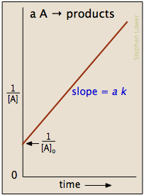
which is easily rearranged into a form of the equation for a straight line and yields plots similar to the one shown below.
The half-life is given by
\[ t_{1/2}=\dfrac{1}{k[A_o]} \nonumber \]
Notice that the half-life of a second-order reaction depends on the initial concentration, in contrast to first-order reactions. For this reason, the concept of half-life for a second-order reaction is far less useful. Reaction rates are discussed in more detail here. Reaction orders are defined here. Here are explanations of zero and first order reactions.
For reactions that follow Equation \ref{case1a} or \ref{case1b}, the rate at which \(\ce{A}\) decreases can be expressed using the differential rate equation.
\[-\dfrac{d[A]}{dt} = k[A]^2 \nonumber \]
The equation can then be rearranged:
\[\dfrac{d[A]}{[A]^2} = -k\,dt \nonumber \]
Since we are interested in the change in concentration of A over a period of time, we integrate between \(t = 0\) and \(t\), the time of interest.
\[ \int_{[A]_o}^{[A]_t} \dfrac{d[A]}{[A]^2} = -k \int_0^t dt \nonumber \]
To solve this, we use the following rule of integration (power rule):
\[\int \dfrac{dx}{x^2} = -\dfrac{1}{x} + constant \nonumber \]
We then obtain the integrated rate equation.
\[\dfrac{1}{[A]_t} - \dfrac{1}{[A]_o} = kt \nonumber \]
Upon rearrangement of the integrated rate equation, we obtain an equation of the line:
\[\dfrac{1}{[A]_t} = kt + \dfrac{1}{[A]_o} \nonumber \]
The crucial part of this process is not understanding precisely how to derive the integrated rate law equation, rather it is important to understand how the equation directly relates to the graph which provides a linear relationship. In this case, and for all second order reactions, the linear plot of \(\dfrac{1}{[A]_t}\) versus time will yield the graph below.
This graph is useful in a variety of ways. If we only know the concentrations at specific times for a reaction, we can attempt to create a graph similar to the one above. If the graph yields a straight line, then the reaction in question must be second order. In addition, with this graph we can find the slope of the line and this slope is \(k\), the reaction constant. The slope can be found be finding the "rise" and then dividing it by the "run" of the line. For an example of how to find the slope, please see the example section below. There are alternative graphs that could be drawn.
The plot of \([A]_t\) versus time would result in a straight line if the reaction were zeroth order. It does, however, yield less information for a second order graph. This is because both the graphs of a first or second order reaction would look like exponential decays. The only obvious difference, as seen in the graph below, is that the concentration of reactants approaches zero more slowly in a second-order, compared to that in a first order reaction.
Case 2: Second Order Reaction with Multiple Reactants
Two different reactants (\(\ce{A}\) and \(\ce{B}\)) combine in a single elementary step:
\[A + B \longrightarrow P \label{case2} \]
The reaction rate for this step can be written as
\[\text{Rate} = - \dfrac{d[A]}{dt}= - \dfrac{d[B]}{dt}= + \dfrac{d[P]}{dt} \nonumber \]
and the rate of loss of reactant \(\ce{A}\)
\[ \dfrac{d[A]}{dt}= - k[A][B] \nonumber \]
where the reaction order with respect to each reactant is 1. This means that when the concentration of reactant A is doubled, the rate of the reaction will double, and quadrupling the concentration of reactant in a separate experiment will quadruple the rate. If we double the concentration of \(\ce{A}\) and quadruple the concentration of \(\ce{B}\) at the same time, then the reaction rate is increased by a factor of 8. This relationship holds true for any varying concentrations of \(\ce{A}\) or \(\ce{B}\).
As before, the rate at which \(A\) decreases can be expressed using the differential rate equation:
\[ \dfrac{d[A]}{dt} = -k[A][B] \nonumber \]
Two situations can be identified.
Situation 2a: \([A]_0 \neq [B]_0\)
Situation 2a is the situation that the initial concentration of the two reactants are not equal. Let \(x\) be the concentration of each species reacted at time \(t\).
Let \( [A]_0 =a\) and \([B]_0 =b\), then \([A]= a-x\) ;\( [B]= b-x\). The expression of rate law becomes:
\[-\dfrac{dx}{dt} = -k([A]_o - x)([B]_o - x)\nonumber \]
which can be rearranged to:
\[\dfrac{dx}{([A]_o - x)([B]_o - x)} = kdt\nonumber \]
We integrate between \(t = 0\) (when \(x = 0\)) and \(t\), the time of interest.
\[ \int_0^x \dfrac{dx}{([A]_o - x)([B]_o - x)} = k \int_0^t dt \nonumber \]
To solve this integral, we use the method of partial fractions.
\[ \int_0^x \dfrac{1}{(a - x)(b -x)}dx = \dfrac{1}{b - a}\left(\ln\dfrac{1}{a - x} - \ln\dfrac{1}{b - x}\right)\nonumber \]
Evaluating the integral gives us:
\[ \int_0^x \dfrac{dx}{([A]_o - x)([B]_o - x)} = \dfrac{1}{[B]_o - [A]_o}\left(\ln\dfrac{[A]_o}{[A]_o - x} - \ln\dfrac{[B]_o}{[B]_o - x}\right) \nonumber \]
Applying the rule of logarithm, the equation simplifies to:
\[\int _0^x \dfrac{dx}{([A]_o - x)([B]_o - x)} = \dfrac{1}{[B]_o - [A]_o} \ln \dfrac{[B][A]_o}{[A][B]_o} \nonumber \]
We then obtain the integrated rate equation (under the condition that [A] and [B] are not equal).
\[ \dfrac{1}{[B]_o - [A]_o}\ln \dfrac{[B][A]_o}{[A][B]_o} = kt \nonumber \]
Upon rearrangement of the integrated rate equation, we obtain:
\[ \ln\dfrac{[B][A]_o}{[A][B]_o} = k([B]_o - [A]_o)t \nonumber \]
Hence, from the last equation, we can see that a linear plot of \(\ln\dfrac{[A]_o[B]}{[A][B]_o}\) versus time is characteristic of second-order reactions.
This graph can be used in the same manner as the graph in the section above or written in the other way:
\[\ln\dfrac{[A]}{[B]} = k([A]_o - [B]_o)t+\ln\dfrac{[A]_o}{[B]_o}\nonumber \]
in form \( y = ax + b\) with a slope of \(a= k([B]_0-[A]_0)\) and a y-intercept of \( b = \ln \dfrac{[A]_0}{[B]_0}\)
Situation 2b: \([A]_0 =[B]_0\)
Because \(A + B \rightarrow P\)
Since \(A\) and \(B\) react with a 1 to 1 stoichiometry, \([A]= [A]_0 -x\) and \([B] = [B]_0 -x\)
at any time \(t\), \([A] = [B]\) and the rate law will be,
\[\text{rate} = k[A][B] = k[A][A] = k[A]^2.\nonumber \]
Thus, it is assumed as the first case!!!
The following chemical equation reaction represents the thermal decomposition of gas \(E\) into \(K\) and \(G\) at 200° C
\[\ce{ 5E(g) -> 4K(g) + G(g)} \nonumber \]
This reaction follows a second order rate law with regards to \(\ce{E}\). For this reaction suppose that the rate constant at 200° C is equivalent to \(4.0 \times 10^{-2} M^{-1}s^{-1}\) and the initial concentration is \(0.050\; M\). What is the initial rate of decomposition of \(\ce{E}\).
Solution
Start by defining the reaction rate in terms of the loss of reactants
\[ \text{Rate (initial)} = - \dfrac{1}{5} \dfrac{d[E]}{dt}\nonumber \]
and then use the rate law to define the rate of loss of \(\ce{E}\)
\[ \dfrac{d[E]}{dt} = -k [A]_i^2 \nonumber \]
We already know \(k\) and \([A]_i\) but we need to figure out \(x\). To do this look at the units of \(k\) and one sees it is M-1s-1 which means the overall reaction is a second order reaction with \(x=2\).
\[\begin{align*} \text{Initial rate} &= (4.0 \times 10^{-2} M^{-1}s^{-1})(0.050\,M)^2 \\[4pt] &= 1 \times 10^{-4} \, Ms^{-1}\end{align*} \nonumber \]
Half-Life
Another characteristic used to determine the order of a reaction from experimental data is the half-life (\(t_{1/2}\)). By definition, the half life of any reaction is the amount of time it takes to consume half of the starting material. For a second-order reaction, the half-life is inversely related to the initial concentration of the reactant (A). For a second-order reaction each half-life is twice as long as the life span of the one before.
Consider the reaction \(2A \rightarrow P\):
We can find an expression for the half-life of a second order reaction by using the previously derived integrated rate equation.
\[\dfrac{1}{[A]_t} - \dfrac{1}{[A]_o} = kt \nonumber \]
Since,
\[[A]_{t_{1/2}} = \dfrac{1}{2}[A]_o \nonumber \]
when \(t = t_{1/2} \).
Our integrated rate equation becomes:
\[\dfrac{1}{\dfrac{1}{2}[A]_o} - \dfrac{1}{[A]_o} = kt_{1/2} \nonumber \]
After a series of algebraic steps,
\[\begin{align*} \dfrac{2}{[A]_o} - \dfrac{1}{[A]_o} &= kt_{1/2} \\[4pt] \dfrac{1}{[A]_o} &= kt_{1/2} \end{align*} \nonumber \]
We obtain the equation for the half-life of a second order reaction:
\[t_{1/2} = \dfrac{1}{k[A]_o} \label{2nd halflife} \]
This inverse relationship suggests that as the initial concentration of reactant is increased, there is a higher probability of the two reactant molecules interacting to form product. Consequently, the reactant will be consumed in a shorter amount of time, i.e. the reaction will have a shorter half-life. This equation also implies that since the half-life is longer when the concentrations are low, species decaying according to second-order kinetics may exist for a longer amount of time if their initial concentrations are small.
Note that for the second scenario in which \(A + B \rightarrow P\), the half-life of the reaction cannot be determined. As stated earlier, \([A]_o\) cannot be equal to \([B]_o\). Hence, the time it takes to consume one-half of A is not the same as the time it takes to consume one-half of B. Because of this, we cannot define a general equation for the half-life of this type of second-order reaction.
If the only reactant is the initial concentration of \(A\), and it is equivalent to \([A]_0=4.50 \times 10^{-5}\,M\) and the reaction is a second order with a rate constant \(k=0.89 M^{-1}s^{-1}\). What is the half-life of this reaction?
Solution
This is a direct application of Equation \ref{2nd halflife}.
\[\begin{align*} \dfrac{1}{k[A]_0} &= \dfrac{1}{(4.50 \times 10^{-5} M)(0.89 M^{-1}{s^{-1})}} \\[4pt] &= 2.50 \times 10^4 \,s \end{align*} \nonumber \]
Summary
| \(2A \rightarrow P\) | \(A + B \rightarrow P\) | |
|---|---|---|
| Differential Form | \(-\dfrac{d[A]}{dt} = k[A]^2\) | \(-\dfrac{d[A]}{dt} = k[A][B]\) |
| Integral Form | \(\dfrac{1}{[A]_t} = kt + \dfrac{1}{[A]_o}\) | \(\dfrac{1}{[B]_o - [A]_o}\ln\dfrac{[B][A]_o}{[A][B]_o} = kt\) |
| Half Life | \(t_{1/2} = \dfrac{1}{k[A]_o}\) | Cannot be easily defined; \(t_{1/2}\) for A and B are different. |
The graph below is the graph that tests if a reaction is second order. The reaction is second order if the graph has a straight line, as is in the example below.
Given the following information, determine the order of the reaction and the value of k, the reaction constant.
| Concentration (M) | Time (s) |
|---|---|
| 1.0 | 10 |
| 0.50 | 20 |
| 0.33 | 30 |
*Hint: Begin by graphing
- Answer
-
Make graphs of concentration vs. time (zeroth order), natural log of concentration vs. time (first order), and one over concentration vs. time (second order). Determine which graph results in a straight line. This graph reflects the order of the reaction. For this problem, the straight line should be in the 3rd graph, meaning the reaction is second order. The numbers should have are:
1/Concentration(M-1) Time (s) 1 10 2 20 3 30 The slope can be found by taking the "rise" over the "run". This means taking two points, (10,1) and (20,2). The "rise" is the vertical distance between the points (2-1=1) and the "run" is the horizontal distance (20-10=10). Therefore the slope is 1/10=0.1. The value of k, therefore, is 0.1 M-2s-1.
Using the following information, determine the half life of this reaction, assuming there is a single reactant.
| Concentration (M) | Time (s) |
|---|---|
| 2.0 | 0 |
| 1.3 | 10 |
| 0.9633 | 20 |
- Answer
-
Determine the order of the reaction and the reaction constant, \(k\), for the reaction using the tactics described in the previous problem. The order of the reaction is second, and the value of k is 0.0269 M-2s-1. Since the reaction order is second, the formula for \(t_{1/2} = k^{-1}[A]_0^{-1}\). This means that the half life of the reaction is 0.0259 seconds.
Given the information from the previous problem, what is the concentration after 5 minutes?
- Answer
-
Convert the time (5 minutes) to seconds. This means the time is 300 seconds. Use the integrated rate law to find the final concentration. The final concentration is 0.1167 M.
References
- Atkins, P. W., & De Paula, J. (2006). Physical Chemistry for the Life Sciences. New York, NY: W. H. Freeman and Company.
- Petrucci, R. H., Harwood, W. S., & Herring, F. G. (2002). General Chemistry: Principles and Modern Applications. Upper Saddle River, NJ: Prentice-Hall, Inc.