
16.15: Solvent Activity Coefficients from Freezing-point Depression Measurements
- Page ID
- 152709

\( \newcommand{\vecs}[1]{\overset { \scriptstyle \rightharpoonup} {\mathbf{#1}} } \)
\( \newcommand{\vecd}[1]{\overset{-\!-\!\rightharpoonup}{\vphantom{a}\smash {#1}}} \)
\( \newcommand{\dsum}{\displaystyle\sum\limits} \)
\( \newcommand{\dint}{\displaystyle\int\limits} \)
\( \newcommand{\dlim}{\displaystyle\lim\limits} \)
\( \newcommand{\id}{\mathrm{id}}\) \( \newcommand{\Span}{\mathrm{span}}\)
( \newcommand{\kernel}{\mathrm{null}\,}\) \( \newcommand{\range}{\mathrm{range}\,}\)
\( \newcommand{\RealPart}{\mathrm{Re}}\) \( \newcommand{\ImaginaryPart}{\mathrm{Im}}\)
\( \newcommand{\Argument}{\mathrm{Arg}}\) \( \newcommand{\norm}[1]{\| #1 \|}\)
\( \newcommand{\inner}[2]{\langle #1, #2 \rangle}\)
\( \newcommand{\Span}{\mathrm{span}}\)
\( \newcommand{\id}{\mathrm{id}}\)
\( \newcommand{\Span}{\mathrm{span}}\)
\( \newcommand{\kernel}{\mathrm{null}\,}\)
\( \newcommand{\range}{\mathrm{range}\,}\)
\( \newcommand{\RealPart}{\mathrm{Re}}\)
\( \newcommand{\ImaginaryPart}{\mathrm{Im}}\)
\( \newcommand{\Argument}{\mathrm{Arg}}\)
\( \newcommand{\norm}[1]{\| #1 \|}\)
\( \newcommand{\inner}[2]{\langle #1, #2 \rangle}\)
\( \newcommand{\Span}{\mathrm{span}}\) \( \newcommand{\AA}{\unicode[.8,0]{x212B}}\)
\( \newcommand{\vectorA}[1]{\vec{#1}} % arrow\)
\( \newcommand{\vectorAt}[1]{\vec{\text{#1}}} % arrow\)
\( \newcommand{\vectorB}[1]{\overset { \scriptstyle \rightharpoonup} {\mathbf{#1}} } \)
\( \newcommand{\vectorC}[1]{\textbf{#1}} \)
\( \newcommand{\vectorD}[1]{\overrightarrow{#1}} \)
\( \newcommand{\vectorDt}[1]{\overrightarrow{\text{#1}}} \)
\( \newcommand{\vectE}[1]{\overset{-\!-\!\rightharpoonup}{\vphantom{a}\smash{\mathbf {#1}}}} \)
\( \newcommand{\vecs}[1]{\overset { \scriptstyle \rightharpoonup} {\mathbf{#1}} } \)
\(\newcommand{\longvect}{\overrightarrow}\)
\( \newcommand{\vecd}[1]{\overset{-\!-\!\rightharpoonup}{\vphantom{a}\smash {#1}}} \)
\(\newcommand{\avec}{\mathbf a}\) \(\newcommand{\bvec}{\mathbf b}\) \(\newcommand{\cvec}{\mathbf c}\) \(\newcommand{\dvec}{\mathbf d}\) \(\newcommand{\dtil}{\widetilde{\mathbf d}}\) \(\newcommand{\evec}{\mathbf e}\) \(\newcommand{\fvec}{\mathbf f}\) \(\newcommand{\nvec}{\mathbf n}\) \(\newcommand{\pvec}{\mathbf p}\) \(\newcommand{\qvec}{\mathbf q}\) \(\newcommand{\svec}{\mathbf s}\) \(\newcommand{\tvec}{\mathbf t}\) \(\newcommand{\uvec}{\mathbf u}\) \(\newcommand{\vvec}{\mathbf v}\) \(\newcommand{\wvec}{\mathbf w}\) \(\newcommand{\xvec}{\mathbf x}\) \(\newcommand{\yvec}{\mathbf y}\) \(\newcommand{\zvec}{\mathbf z}\) \(\newcommand{\rvec}{\mathbf r}\) \(\newcommand{\mvec}{\mathbf m}\) \(\newcommand{\zerovec}{\mathbf 0}\) \(\newcommand{\onevec}{\mathbf 1}\) \(\newcommand{\real}{\mathbb R}\) \(\newcommand{\twovec}[2]{\left[\begin{array}{r}#1 \\ #2 \end{array}\right]}\) \(\newcommand{\ctwovec}[2]{\left[\begin{array}{c}#1 \\ #2 \end{array}\right]}\) \(\newcommand{\threevec}[3]{\left[\begin{array}{r}#1 \\ #2 \\ #3 \end{array}\right]}\) \(\newcommand{\cthreevec}[3]{\left[\begin{array}{c}#1 \\ #2 \\ #3 \end{array}\right]}\) \(\newcommand{\fourvec}[4]{\left[\begin{array}{r}#1 \\ #2 \\ #3 \\ #4 \end{array}\right]}\) \(\newcommand{\cfourvec}[4]{\left[\begin{array}{c}#1 \\ #2 \\ #3 \\ #4 \end{array}\right]}\) \(\newcommand{\fivevec}[5]{\left[\begin{array}{r}#1 \\ #2 \\ #3 \\ #4 \\ #5 \\ \end{array}\right]}\) \(\newcommand{\cfivevec}[5]{\left[\begin{array}{c}#1 \\ #2 \\ #3 \\ #4 \\ #5 \\ \end{array}\right]}\) \(\newcommand{\mattwo}[4]{\left[\begin{array}{rr}#1 \amp #2 \\ #3 \amp #4 \\ \end{array}\right]}\) \(\newcommand{\laspan}[1]{\text{Span}\{#1\}}\) \(\newcommand{\bcal}{\cal B}\) \(\newcommand{\ccal}{\cal C}\) \(\newcommand{\scal}{\cal S}\) \(\newcommand{\wcal}{\cal W}\) \(\newcommand{\ecal}{\cal E}\) \(\newcommand{\coords}[2]{\left\{#1\right\}_{#2}}\) \(\newcommand{\gray}[1]{\color{gray}{#1}}\) \(\newcommand{\lgray}[1]{\color{lightgray}{#1}}\) \(\newcommand{\rank}{\operatorname{rank}}\) \(\newcommand{\row}{\text{Row}}\) \(\newcommand{\col}{\text{Col}}\) \(\renewcommand{\row}{\text{Row}}\) \(\newcommand{\nul}{\text{Nul}}\) \(\newcommand{\var}{\text{Var}}\) \(\newcommand{\corr}{\text{corr}}\) \(\newcommand{\len}[1]{\left|#1\right|}\) \(\newcommand{\bbar}{\overline{\bvec}}\) \(\newcommand{\bhat}{\widehat{\bvec}}\) \(\newcommand{\bperp}{\bvec^\perp}\) \(\newcommand{\xhat}{\widehat{\xvec}}\) \(\newcommand{\vhat}{\widehat{\vvec}}\) \(\newcommand{\uhat}{\widehat{\uvec}}\) \(\newcommand{\what}{\widehat{\wvec}}\) \(\newcommand{\Sighat}{\widehat{\Sigma}}\) \(\newcommand{\lt}{<}\) \(\newcommand{\gt}{>}\) \(\newcommand{\amp}{&}\) \(\definecolor{fillinmathshade}{gray}{0.9}\)The analysis of freezing-point depression that we present in Section 16.11 introduces a number of simplifying assumptions. We now undertake a more rigorous analysis of this phenomenon. This analysis is of practical importance. Measuring the freezing-point depression of a solution is one way that we can determine the activity and the activity coefficient of the solvent component. As we see in Section 16.7, if we have activity coefficients for the solvent over a range of solute concentrations, we can use the Gibbs-Duhem equation to find activity coefficients for the solute. Freezing-point depression measurements have been used extensively to determine the activity coefficients of aqueous solutes by measuring the activity of water in their solutions.
As in our earlier discussion of freezing-point depression, the equilibrium system is a solution of solute \(A\) in solvent \(B\), which is in phase equilibrium with pure solid solvent \(B\). Our present objective is to determine the activity of the solvent in its solutions at the melting point of the pure solvent. Having obtained this information, we can use the Gibbs-Duhem relationship to find the activity of the solute, as a function of solute concentration, at the melting point of the pure solvent. Once we have the solute activity at the melting point of the pure solvent, we can use the methods developed in Section 14.14 to find the solute activity in a solution at any higher temperature.
In Section 14.14, we find the temperature dependence of the natural logarithm of the chemical activity of a component of a solution. For a particular choice of activity standard states and enthalpy reference states, we develop a method to obtain the experimental data that we need to apply this equation. For brevity, let us refer to these choices as the infinite dilution standard states. In order to determine the activity of a solvent in its solutions at the melting point of the pure solvent, it is useful to define an additional standard state for the solvent. At temperatures below the normal melting point, which we again designate as \(T_F\), we let the activity standard state of the solvent be pure solid \(B\). Above the melting point, we use the infinite dilution standard state that we define in Section 14.14; that is, we let the activity standard state of the solvent be pure liquid solvent \(B\).
At and below the melting point, \(T_F\), the activity standard state for the solvent, \(B\), is pure solid \(B\). At and above the melting point, the activity standard state for the solvent is pure liquid \(B\). At the melting point, pure solid solvent is in equilibrium with pure liquid solvent, which is also the solvent in an infinitely dilute solution. At \(T_F\), the activity standard state chemical potentials of the pure solid solvent, the pure liquid solvent, and the solvent in an infinitely dilute solution are all the same. It follows that the value that we obtain for the activity of the solvent at \(T_F\), for any particular solution, will be the same whether we determine it from measurements below \(T_F\) using the pure solid standard state or from measurements above \(T_F\) using the infinitely dilute solution standard state.
Now let us consider the chemical potential of liquid solvent \(B\) in a solution whose composition is specified by the molality of solute \(A\), \({\underline{m}}_A\), when the activity standard state is pure solid \(B\). We want to find this chemical potential at temperatures in the range \(T_{fp}
\[{\mu }_B\left(\mathrm{solution},\ {\underline{m}}_A,T\right) \nonumber \] \[={\widetilde{\mu }}^o_B\left(\mathrm{pure\ solid},\ T\right)+RT{ \ln {\tilde{a}}_B\ }\left(\mathrm{solution},\ {\underline{m}}_A,T\right) \nonumber \]
Using the Gibbs-Helmholtz equation, we obtain
\[{\left(\frac{\partial { \ln {\tilde{a}}_B\ }\left(\mathrm{solution},\ {\underline{m}}_A,T\right)}{\partial T}\right)}_{P,{\underline{m}}_A} \nonumber \]
\[\ \ \ \ =\frac{-{\overline{H}}_B\left(\mathrm{solution},\ {\underline{m}}_A,T\right)}{RT^2}+\frac{{\tilde{H}}^o_B\left(T\right)}{RT^2} \nonumber \] \[=\frac{-\left[{\overline{H}}_B\left(\mathrm{solution},\ {\underline{m}}_A,T\right)-{\overline{H}}^{\textrm{⦁}}_B\left(\mathrm{solid},T\right)\right]}{RT^2} \nonumber \]
where we have \({\tilde{H}}^o_B\left(T\right)={\overline{H}}^{\textrm{⦁}}_B\left(\mathrm{solid},T\right)\), because pure solid \(B\) is the activity standard state. Using the ideas developed in Section 14.14, we can use the thermochemical cycle shown in Figure 10 to evaluate
\[{\overline{H}}_B\left(\mathrm{solution},\ {\underline{m}}_A,T\right)-{\overline{H}}^{\textrm{⦁}}_B\left(\mathrm{solid},T\right) \nonumber \]
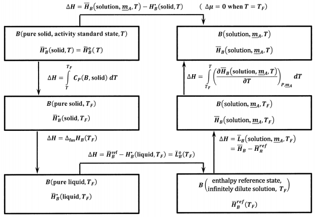
In this cycle, \({\Delta }_{\mathrm{fus}}{\overline{H}}_B\left(T_F\right)\) is the molar enthalpy of fusion of pure \(B\) at the melting point, \(T_F\). \({\overline{L}}_B\left(\mathrm{solution},\ {\underline{m}}_A,T\right)\) is the relative partial molar enthalpy of \(B\) at \(T_F\) in a solution whose composition is specified by \({\underline{m}}_A\). The only new quantity in this cycle is
\[\int^T_{T_f}{{\left(\frac{\partial {\overline{H}}_B\left(\mathrm{solution},\ {\underline{m}}_A,T\right)}{\partial T}\right)}_{P,{\underline{m}}_A}dT} \nonumber \] We can use the relative partial molar enthalpy of the solution to find it. By definition,
\[{\overline{L}}_B\left(\mathrm{solution},\ {\underline{m}}_A,T\right) \nonumber \] \[={\left(\frac{\partial H\left(\mathrm{solution},\ {\underline{m}}_A,T\right)}{\partial n_B}\right)}_{P,T,n_A}-{\overline{H}}^{\mathrm{ref}}_B\left(T\right) \nonumber \]
or, dropping the parenthetical information,
\[{\overline{L}}_B={\overline{H}}_B-{\overline{H}}^{\mathrm{ref}}_B\left(T\right) \nonumber \]
so that \[{\left(\frac{{\partial \overline{L}}_B}{\partial T}\right)}_P={\left(\frac{\partial {\overline{H}}_B}{\partial T}\right)}_P-{\left(\frac{\partial {\overline{H}}^{\mathrm{ref}}_B}{\partial T}\right)}_P \nonumber \]
In Section 14.14, we introduce the relative partial molar heat capacity,
\[{\overline{J}}_B\left(T\right)={\left(\frac{{\partial \overline{L}}_B}{\partial T}\right)}_P \nonumber \]
Since the infinitely dilute solution is the enthalpy reference state for \(B\) in solution, we expect the molar enthalpy of pure liquid \(B\) to be a good approximation to the partial molar enthalpy of liquid \(B\) in the enthalpy reference state. Then, \({\left({\partial {\overline{H}}^{\mathrm{ref}}_B}/{\partial T}\right)}_P\) is just the molar heat capacity of pure liquid \(B\), \(C_P\left(B,\mathrm{liquid},T\right)\). (See problem 16-11.) We find
\[{\left(\frac{\partial {\overline{H}}_B}{\partial T}\right)}_P={\overline{J}}_B\left(T\right)+C_P\left(B,\mathrm{liquid},T\right) \nonumber \]
Using this result, the enthalpy changes around the cycle in Figure 10 yield
\[{\overline{H}}_B\left(\mathrm{solution},\ {\underline{m}}_A,T\right)-{\overline{H}}^{\textrm{⦁}}_B\left(\mathrm{solid},T\right) \nonumber \]
\[=\int^{T_F}_T{C_P\left(B,\mathrm{solid},T\right)}dT+{\Delta }_{\mathrm{fus}}{\overline{H}}_B\left(T_F\right)-L^o_B\left(T_F\right)+{\overline{L}}_B\left({\underline{m}}_A,T_F\right)+\int^T_{T_F}{\left[{\overline{J}}_B\left(T\right)+\mathrm{\ }C_P\left(B,\mathrm{liquid},T\right)\right]}dT \nonumber \]
\[={\Delta }_{\mathrm{fus}}{\overline{H}}_B\left(T_F\right)+{\overline{L}}_B\left({\underline{m}}_A,T_F\right)-L^o_B\left(T_F\right)-\int^{T_F}_T{\left[C_P\left(B,\mathrm{liquid},T\right)-C_P\left(B,\mathrm{solid},T\right)+{\overline{J}}_B\right]}dT \nonumber \]
Since we know how to determine \({\overline{J}}_B\) and the heat capacities as functions of temperature, we can evaluate this integral to obtain a function of temperature. For present purposes, let us assume that \({\overline{J}}_B\) and the heat capacities are essentially constant and introduce the abbreviation \(\Delta C_P=C_P\left(B,\mathrm{liquid},T\right)-C_P\left(B,\mathrm{solid},T\right)\), so that \[\int^{T_F}_T{\left[C_P\left(B,\mathrm{liquid},T\right)-C_P\left(B,\mathrm{solid},T\right)+{\overline{J}}_B\right]}dT=\left(\Delta C_P+{\overline{J}}_B\right)\left(T_F-T\right) \nonumber \]
The temperature derivative of \({ \ln {\tilde{a}}_B\ }\left(\mathrm{solution},\ {\underline{m}}_A,T\right)\) becomes
\[{\left(\frac{\partial { \ln {\tilde{a}}_B\ }\left(\mathrm{solution},\ {\underline{m}}_A,T\right)}{\partial T}\right)}_{P,{\underline{m}}_A} \nonumber \] \[=\frac{-{\Delta }_{\mathrm{fus}}{\overline{H}}_B\left(T_F\right)-{\overline{L}}_B\left({\underline{m}}_A,T_F\right)+L^o_B\left(T_F\right)}{RT^2}+\frac{\left(\Delta C_P+{\overline{J}}_B\right)\left(T_F-T\right)}{RT^2} \nonumber \]
\(T_{fp}\) is the freezing point of the solution whose composition is specified by \({\underline{m}}_A\). At \(T_{fp}\) the solvent in this solution is at equilibrium with pure solid solvent. Hence, the chemical potential of the solution solvent is equal to that of the pure-solid solvent. Then, because the pure solid is the activity standard state for both solution solvent and pure-solid solvent at \(T_{fp}\), the activity of the solution solvent is equal to that of the pure-solid solvent. Because the pure solid is the activity standard state, the solvent activity is unity at \(T_{fp}\). This means that we can integrate the temperature derivative from \(T_{fp}\) to \(T_F\) to obtain
\[\begin{aligned} \int^{T_F}_{T_{fp}} d ~ \ln \tilde{a}_B \left(\mathrm{solution},\ {\underline{m}}_A,T\right) & ~ \\ ~ & = \ln \tilde{a}_B \left(\mathrm{solution},\ {\underline{m}}_A,T_F\right) \\ ~ & = \left( \frac{\Delta _{\text{fus}} \overline{H}_B \left(T_F \right)+ \overline{L}_B \left( \underline{m}_A, T_F \right) +L^o_B\left(T_F\right)}{R} \right) \left(\frac{1}{T_F}-\frac{1}{T_{fp}}\right) -\left(\frac{\Delta C_P+ \overline{J}_B}{R}\right) \left(1-\frac{T_F}{T_{fp}}+ \ln \left(\frac{T_F}{T_{fp}} \right) \right) \end{aligned} \nonumber \]
Thus, from the measured freezing point of a solution whose composition is specified by \({\underline{m}}_A\), we can calculate the activity of the solvent in that solution at \(T_F\).
Several features of this result warrant mention. It is important to remember that we obtained it by assuming that \(\Delta C_P+{\overline{J}}_B\left(T\right)\) is a constant. This is usually a good assumption. It is customary to express experimental results as values of the freezing-point depression, \(\Delta T=T_F-T_{fp}\). The activity equation becomes
\[\begin{aligned} \ln \tilde{a}_B \left(\mathrm{solution}, \underline{m}_A,T_F\right) & ~ \\ ~ & =-\left(\frac{\Delta _{\mathrm{fus}} \overline{H}_B\left(T_F\right)+\overline{L}_B\left( \underline{m}_A,T_F\right)+L^o_B\left(T_F\right)}{RT_FT_{fp}}\right)\Delta T \\ ~ & +\left(\frac{\Delta C_P+{\overline{J}}_B}{R}\right)\left(\frac{\Delta T}{T_{fp}}-{ \ln \left(1+\frac{\Delta T}{T_{fp}}\right)\ }\right) \end{aligned} \nonumber \]
The terms involving \({\overline{L}}_B\), \(L^o_B\), \(\Delta C_P\), and \({\overline{J}}_B\) are often negligible, particularly when the solute concentration is low. When \({T_F}/{T_{fp}\approx 1}\), that is, when the freezing-point depression is small, the coefficient of \(\Delta C_P+{\overline{J}}_B\) is approximately zero. When these approximations apply, the activity equation is approximated by
\[{ \ln {\tilde{a}}_B\ }\left(\mathrm{solution},\ {\underline{m}}_A,T_F\right)=-\left(\frac{{\Delta }_{\mathrm{fus}}{\overline{H}}_B\left(T_F\right)}{RT^2_F}\right)\Delta T \nonumber \]