
16.7: Finding the Activity of a Solute from the Activity of the Solvent
- Page ID
- 152701

\( \newcommand{\vecs}[1]{\overset { \scriptstyle \rightharpoonup} {\mathbf{#1}} } \)
\( \newcommand{\vecd}[1]{\overset{-\!-\!\rightharpoonup}{\vphantom{a}\smash {#1}}} \)
\( \newcommand{\id}{\mathrm{id}}\) \( \newcommand{\Span}{\mathrm{span}}\)
( \newcommand{\kernel}{\mathrm{null}\,}\) \( \newcommand{\range}{\mathrm{range}\,}\)
\( \newcommand{\RealPart}{\mathrm{Re}}\) \( \newcommand{\ImaginaryPart}{\mathrm{Im}}\)
\( \newcommand{\Argument}{\mathrm{Arg}}\) \( \newcommand{\norm}[1]{\| #1 \|}\)
\( \newcommand{\inner}[2]{\langle #1, #2 \rangle}\)
\( \newcommand{\Span}{\mathrm{span}}\)
\( \newcommand{\id}{\mathrm{id}}\)
\( \newcommand{\Span}{\mathrm{span}}\)
\( \newcommand{\kernel}{\mathrm{null}\,}\)
\( \newcommand{\range}{\mathrm{range}\,}\)
\( \newcommand{\RealPart}{\mathrm{Re}}\)
\( \newcommand{\ImaginaryPart}{\mathrm{Im}}\)
\( \newcommand{\Argument}{\mathrm{Arg}}\)
\( \newcommand{\norm}[1]{\| #1 \|}\)
\( \newcommand{\inner}[2]{\langle #1, #2 \rangle}\)
\( \newcommand{\Span}{\mathrm{span}}\) \( \newcommand{\AA}{\unicode[.8,0]{x212B}}\)
\( \newcommand{\vectorA}[1]{\vec{#1}} % arrow\)
\( \newcommand{\vectorAt}[1]{\vec{\text{#1}}} % arrow\)
\( \newcommand{\vectorB}[1]{\overset { \scriptstyle \rightharpoonup} {\mathbf{#1}} } \)
\( \newcommand{\vectorC}[1]{\textbf{#1}} \)
\( \newcommand{\vectorD}[1]{\overrightarrow{#1}} \)
\( \newcommand{\vectorDt}[1]{\overrightarrow{\text{#1}}} \)
\( \newcommand{\vectE}[1]{\overset{-\!-\!\rightharpoonup}{\vphantom{a}\smash{\mathbf {#1}}}} \)
\( \newcommand{\vecs}[1]{\overset { \scriptstyle \rightharpoonup} {\mathbf{#1}} } \)
\( \newcommand{\vecd}[1]{\overset{-\!-\!\rightharpoonup}{\vphantom{a}\smash {#1}}} \)
\(\newcommand{\avec}{\mathbf a}\) \(\newcommand{\bvec}{\mathbf b}\) \(\newcommand{\cvec}{\mathbf c}\) \(\newcommand{\dvec}{\mathbf d}\) \(\newcommand{\dtil}{\widetilde{\mathbf d}}\) \(\newcommand{\evec}{\mathbf e}\) \(\newcommand{\fvec}{\mathbf f}\) \(\newcommand{\nvec}{\mathbf n}\) \(\newcommand{\pvec}{\mathbf p}\) \(\newcommand{\qvec}{\mathbf q}\) \(\newcommand{\svec}{\mathbf s}\) \(\newcommand{\tvec}{\mathbf t}\) \(\newcommand{\uvec}{\mathbf u}\) \(\newcommand{\vvec}{\mathbf v}\) \(\newcommand{\wvec}{\mathbf w}\) \(\newcommand{\xvec}{\mathbf x}\) \(\newcommand{\yvec}{\mathbf y}\) \(\newcommand{\zvec}{\mathbf z}\) \(\newcommand{\rvec}{\mathbf r}\) \(\newcommand{\mvec}{\mathbf m}\) \(\newcommand{\zerovec}{\mathbf 0}\) \(\newcommand{\onevec}{\mathbf 1}\) \(\newcommand{\real}{\mathbb R}\) \(\newcommand{\twovec}[2]{\left[\begin{array}{r}#1 \\ #2 \end{array}\right]}\) \(\newcommand{\ctwovec}[2]{\left[\begin{array}{c}#1 \\ #2 \end{array}\right]}\) \(\newcommand{\threevec}[3]{\left[\begin{array}{r}#1 \\ #2 \\ #3 \end{array}\right]}\) \(\newcommand{\cthreevec}[3]{\left[\begin{array}{c}#1 \\ #2 \\ #3 \end{array}\right]}\) \(\newcommand{\fourvec}[4]{\left[\begin{array}{r}#1 \\ #2 \\ #3 \\ #4 \end{array}\right]}\) \(\newcommand{\cfourvec}[4]{\left[\begin{array}{c}#1 \\ #2 \\ #3 \\ #4 \end{array}\right]}\) \(\newcommand{\fivevec}[5]{\left[\begin{array}{r}#1 \\ #2 \\ #3 \\ #4 \\ #5 \\ \end{array}\right]}\) \(\newcommand{\cfivevec}[5]{\left[\begin{array}{c}#1 \\ #2 \\ #3 \\ #4 \\ #5 \\ \end{array}\right]}\) \(\newcommand{\mattwo}[4]{\left[\begin{array}{rr}#1 \amp #2 \\ #3 \amp #4 \\ \end{array}\right]}\) \(\newcommand{\laspan}[1]{\text{Span}\{#1\}}\) \(\newcommand{\bcal}{\cal B}\) \(\newcommand{\ccal}{\cal C}\) \(\newcommand{\scal}{\cal S}\) \(\newcommand{\wcal}{\cal W}\) \(\newcommand{\ecal}{\cal E}\) \(\newcommand{\coords}[2]{\left\{#1\right\}_{#2}}\) \(\newcommand{\gray}[1]{\color{gray}{#1}}\) \(\newcommand{\lgray}[1]{\color{lightgray}{#1}}\) \(\newcommand{\rank}{\operatorname{rank}}\) \(\newcommand{\row}{\text{Row}}\) \(\newcommand{\col}{\text{Col}}\) \(\renewcommand{\row}{\text{Row}}\) \(\newcommand{\nul}{\text{Nul}}\) \(\newcommand{\var}{\text{Var}}\) \(\newcommand{\corr}{\text{corr}}\) \(\newcommand{\len}[1]{\left|#1\right|}\) \(\newcommand{\bbar}{\overline{\bvec}}\) \(\newcommand{\bhat}{\widehat{\bvec}}\) \(\newcommand{\bperp}{\bvec^\perp}\) \(\newcommand{\xhat}{\widehat{\xvec}}\) \(\newcommand{\vhat}{\widehat{\vvec}}\) \(\newcommand{\uhat}{\widehat{\uvec}}\) \(\newcommand{\what}{\widehat{\wvec}}\) \(\newcommand{\Sighat}{\widehat{\Sigma}}\) \(\newcommand{\lt}{<}\) \(\newcommand{\gt}{>}\) \(\newcommand{\amp}{&}\) \(\definecolor{fillinmathshade}{gray}{0.9}\)We have seen that the activity of any component of an equilibrium system contains information about the activities of all the other components. From
\[d\mu =-\overline{S}dT+\overline{V}P+RTd{ \ln \tilde{a}\ }\nonumber \]
and the Gibbs-Duhem equation, we can find a general relationship among the activities. Substituting \(d{\mu }_A\) and \(d{\mu }_B\) into the Gibbs-Duhem equation, we have, for a two-component solution,
\[ \begin{align*} -SdT+VdP &=n_Ad{\mu }_A+n_Bd{\mu }_B \\[4pt]&= n_A\left(-{\overline{S}}_AdT+{\overline{V}}_AP+RTd{ \ln {\tilde{a}}_A\ }\right)+n_B\left(-{\overline{S}}_BdT+{\overline{V}}_BP+RTd{ \ln {\tilde{a}}_B\ }\right) \\[4pt]&= -\left(n_A{\overline{S}}_A+n_B{\overline{S}}_B\right)dT + \left(n_A{\overline{V}}_A+n_B{\overline{V}}_B\right)dP + n_ARTd{ \ln {\tilde{a}}_A\ }+n_BRTd{ \ln {\tilde{a}}_B\ }\end{align*} \nonumber \]
Since \(S=n_A{\overline{S}}_A+n_B{\overline{S}}_B\) and \(V=n_A{\overline{V}}_A+n_B{\overline{V}}_B\), this simplifies to
\[0=n_Ad{ \ln {\tilde{a}}_A\ }+n_Bd{ \ln {\tilde{a}}_B\ }\nonumber \]
or, dividing by \(n_A+n_B\),
\[0=y_Ad{ \ln {\tilde{a}}_A\ }+y_Bd{ \ln {\tilde{a}}_B\ }\nonumber \]
For simplicity, let us consider a system in which a non-volatile solute, \(A\), is dissolved in a volatile solvent, \(B\). Measuring the pressure of the system and applying the equations that we developed in Section 16.1 for volatile component \(A\) to the volatile solvent, \(B\), in the present system, we can determine the activity of the solvent, \(B\). Let us use mole fractions to measure concentrations and take pure liquid \(B\) at its equilibrium vapor pressure as the activity standard state for both liquid- and gas-phase \(B\). When \(B\) is in its standard state, we have \(x_A=0\), \(x_B=1\), and \({\overline{V}}_B\left(g\right)={\overline{V}}^{\textrm{⦁}}_B\left(g\right)\). Then, since the solute is non-volatile, we can determine the activity of the solvent, \(B\), from the pressure of the system. We have
\[{ \ln \left[{\tilde{a}}_B\left(P,y_A,y_B\right)\right]=\ }RT{ \ln \left[\frac{P}{P^{\textrm{⦁}}_B}\right]-\int^P_{P^{\textrm{⦁}}_B}{\left(\frac{{\overline{V}}^{\textrm{⦁}}_B \left(g\right)}{RT}-\frac{1}{P}\right)}\ }dP\nonumber \]
Assuming that the integral makes a negligible contribution to the activity, we have
\[{\tilde{a}}_B\left(P,y_A,y_B\right)={\tilde{a}}_B=y_B\gamma_B\left(P,y_A,y_B\right)=\frac{P}{P^{\textrm{⦁}}_B}\nonumber \] (solvent)
so that
\[\gamma_B\left(P,y_A,y_B\right)=\gamma_B=\frac{P}{y_BP^{\textrm{⦁}}_B}\nonumber \] (solvent)
Since the gas-phase concentration of \(A\) is immeasurably small, we must determine its activity indirectly. Let the standard state for solute activity be the hypothetical pure liquid, \(y_A=1\), whose equilibrium vapor pressure is equal to the Henry’s law constant of solute \(A\). (We can determine the solute’s activity without measuring its Henry’s law constant.) We have
\[{\mu }_A\left(P,y_A,y_B\right)={\widetilde{\mu }}^o_A\left(Hyp\ \ell ,{\textrm{ҝ}}_A\right)+RT{ \ln \left[{\tilde{a}}_A\left(P,y_A,y_B\right)\right]\ }\nonumber \]
where
\[{\tilde{a}}_A\left(P,y_A,y_B\right)={\tilde{a}}_A=y_A\gamma_A\nonumber \] (solute)
Since we are able to measure the activity of the solvent, we can determine the activity of the solute from the relationship \(0=y_Ad{ \ln {\tilde{a}}_A\ }+y_Bd{ \ln {\tilde{a}}_B\ }\). Rearranging, we have
\[d{ \ln {\tilde{a}}_A\ }=-\frac{y_B}{y_A}d{ \ln {\tilde{a}}_B\ }=-\left(\frac{{1-y}_A}{y_A}\right)d{ \ln {\tilde{a}}_B\ }\nonumber \]
For two solutions in which the mole fractions of \(A\) are \(y_A\) and \(y^{\#}_A\), and in which the activities of \(A\) and \(B\) are \({\tilde{a}}_A\), \({\tilde{a}}_B\), \({\tilde{a}}^{\#}_A\), and \({\tilde{a}}^{\#}_B\), we have
\[ \ln \frac{\tilde{a}_A}{\tilde{a}^{\#}_A}=-\int^{y_A}_{y^{\#}_A} \left(\frac{1-y_A}{y_A}\right)d \ln \tilde{a}_B\nonumber \]
Graphically, the integral is the area under a plot of \(-{\left(1-y_A\right)}/{y_A}\) versus \({ \ln {\tilde{a}}_B\ }\), from \(y^{\#}_A\) to \(y_A\).
Typically, we are interested in solutions for which \(y_A\ll y_B\). In the limit as the solution becomes very dilute, the activity, mole fraction, and activity coefficient of the solvent, \(B\), all approach unity: \({\tilde{a}}_B\to 1\), \(y_B\to 1\), and \(\gamma_B\to 1\). The activity of the solute, \(A\), approaches the mole fraction of \(A\). As a matter of experience, the approach is asymptotic: as the mole fraction approaches zero, \(y_A\to 0\), the solute activity coefficient approaches unity, \(\gamma_A\to 1\), and does so asymptotically, so that \({\tilde{a}}_A\to y_A\). For dilute solutions, \({ \ln {\tilde{a}}_A\to -\infty \ }\) and \({ \ln \gamma_A\to 0\ }\) asymptotically. In consequence,
\[{\mathop{\mathrm{lim}}_{y_A\to 0} \left(d{ \ln \gamma_A\ }\right)\ }=0\nonumber \]
Because the activity coefficient approaches a finite limit while the activity does not, we can express the solute’s activity most simply by finding the solute’s activity coefficient. Since \({\tilde{a}}_A=y_A\gamma_A\) and \({\tilde{a}}_B=y_B\gamma_B=\left(1-y_A\right)\gamma_B\), we have
\[\begin{align*} 0 &=y_Ad{ \ln {\tilde{a}}_A\ }+y_Bd{ \ln {\tilde{a}}_B\ } \\[4pt] &=y_Ad{ \ln y_A\gamma_A\ }+y_Bd{ \ln y_B\gamma_B\ }=y_Ad{ \ln y_A\ }+y_Ad{ \ln \gamma_A\ }+y_Bd{ \ln y_B\ }+y_Bd{ \ln \gamma_B\ } \\[4pt]&=\left(dy_A+dy_B\right)+y_Ad{ \ln \gamma_A\ }+y_Bd{ \ln \gamma_B\ }=y_Ad{ \ln \gamma_A\ }+y_Bd{ \ln \gamma_B\ }\end{align*} \nonumber \]
(Since \(y_A+y_B=1\), we have \({dy}_A+{dy}_B=0\).) We can rearrange this to
\[d{ \ln \gamma_A\ }=-\left(\frac{{1-y}_A}{y_A}\right)d{ \ln \gamma_B\ }\nonumber \]
As the solute concentration approaches zero, \({\left(1-y_A\right)}/{y_A}\) becomes arbitrarily large. However, since \({\mathop{\mathrm{lim}}_{y_A\to 0} \left(d{ \ln \gamma_A\ }\right)\ }=0\), it follows that
\[{\mathop{\mathrm{lim}}_{y_A\to 0} d{ \ln \gamma_B\ }\ }=0\nonumber \]
We see that the solvent activity coefficient also approaches unity asymptotically as the solute concentration goes to zero. The solute activity coefficient at any \(y_A>0\) is then given by
\[\int^{y_A}_0 d \ln \left[\gamma_A\left(y_A\right)\right] \ln \left[\gamma_A\left(y_A\right)\right] \int^{y_A}_0 -\left(\frac{1-y_A}{y_A}\right)d \ln \left[\gamma_B\left(y_A\right)\right]\nonumber \]
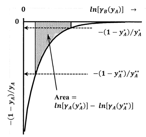
As sketched in Figure 6, the latter integral is the area under a graph of \({-\left(1-y_A\right)}/{y_A}\) versus \({ \ln \left[\gamma_B\left(y_A\right)\right]\ }\), between \(y_A=0\) and \(y_A\). Since \(\gamma_A\left(y_A\right)\to 1\) as \(y_A\to 0\), this integral must remain finite even though \({-\left(1-y_A\right)}/{y_A}\to -\infty\) as \(y_A\to 0\). This can occur, because \({\mathop{\mathrm{lim}}_{y_A\to 0} d{ \ln \gamma_B\ }\ }=0\), as we observe above. Nevertheless, the fact that the integrand is unbounded can limit the accuracy of the necessary integration. For accurate measurement of the solute activity coefficient, it is important to obtain solvent-activity data at the lowest possible solute concentration.
The most desirable situation is to collect solvent-activity data down to solute concentrations at which the solvent activity coefficient, \(\gamma_B\), becomes unity. If \(\gamma_B\left(y^{\#}_A\right)=1\) when the solute concentration is \(y^{\#}_A\), \({ \ln \left[\gamma_A\left(y_A\right)\right]\ }\) can be evaluated with \(y^{\#}_A\), rather than zero, as the lower limit of integration. In some cases, \({ \ln \left[\gamma_A\left(y^{\triangle }_A\right)\right]\ }\) may be known from some other measurement at a particular concentration, \(y^{\triangle }_A\); if so, we can find \({ \ln \left[\gamma_A\left(y_A\right)\right]\ }\) by carrying out the numerical integration between the limits \(y^{\triangle }_A\) and \(y_A\).
If the measurement of \(\gamma_B\) cannot be extended to values of \(y_A\) at which \(\gamma_B\left(y_A\right)=1\), we must find an empirical function, call it \(f\left(y_A\right)\), that fits the experimental values of \({ \ln \left[\gamma_B\left(y_A\right)\right]\ }\), for the smallest values of \(y_A\). (That is, the empirical function is \({f\left(y_A\right)\mathrm{=ln} \left[\gamma_B\left(y_A\right)\right]\ }\).) The differential of \(f\left(y_A\right)\) is then a mathematical model for \(d{ \ln \left[\gamma_B\left(y_A\right)\right]\ }\) over the region of low solute concentrations. Letting \(y^{\#}_A\) be the smallest solute concentration for which the solvent activity can be determined, we can integrate, using the function for \(d{ \ln \left[\gamma_B\left(y_A\right)\right]\ }\) that we derive from this model, to estimate \({ \ln \left[\gamma_B\left(y^{\#}_A\right)\right]\ }\). Uncertainty about the accuracy of the mathematical model becomes a significant source of uncertainty in the calculated values of \(\gamma_A\).
Of course, if we can find an analytical function that provides a good mathematical model for all of the solvent-activity data, the differential of this function can be used in the integral to evaluate \({ \ln \left[\gamma_A\left(y_A\right)\right]\ }\) over the entire range of the experimental data. If necessary, the evaluation of this integral can be accomplished using numerical methods.
It is essential that any empirical function, \({f\left(y_A\right)\mathrm{=ln} \left[\gamma_B\left(y_A\right)\right]\ }\), have the correct mathematical properties over the concentration range to which it is applied. If it is to be used to extend the integration to \(y_A=0\), \(f\left(y_A\right)\) must satisfy \(f\left(0\right)=0\) and \(df\left(0\right)=0\). This is a significant condition. For example, consider the approximation
\[f\left(y_A\right)={ \ln \left[\gamma_B\left(y_A\right)\right]\ }=c_By^{{\alpha }_B}_A\nonumber \]
This model gives
\[\frac{d{ \ln \left[\gamma_A\left(y_A\right)\right]\ }}{dy_A}={-\left(1-y_A\right)c}_B{\alpha }_By^{{\alpha }_B-2}_A\nonumber \] and \[{\mathop{\mathrm{lim}}_{y_A\to 0} \frac{d{ \ln \left[\gamma_A\left(y_A\right)\right]\ }}{dy_A}\ }=0\nonumber \]
requires \({\alpha }_B>2\).