16.1: Solutions Whose Components are in Equilibrium with Their Own Gases

One way to find activities is to find the composition and pressure of the gas phase that is in equilibrium with the solution. If the gases are not ideal, we also need experimental data on the partial molar volumes of the components in the gas phase. Collecting such data is feasible for solutions of volatile molecular liquids. For solutions of electrolytes or other non-volatile components, other methods are required.

Figure 1. Equilibrium mole fractions in gas and liquid phases.

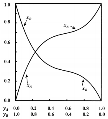
The curves sketched in Figure 1 describe a system containing components \(A\) and \(B\). The mole fractions in the solution and the mole fractions in the gas are related in a non-linear way. Let the mole fractions in the gas be \(x_A\) and \(x_B\); let those in the solution be \(y_A\) and \(y_B\). We have \(x_A+x_B=1\) and \(y_A+y_B=1\). At equilibrium, both phases are at the same pressure, \(P\).

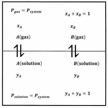
We imagine obtaining the data we need about this system by preparing many mixtures of \(A\) and \(B\). Beginning with an entirely liquid system at some applied pressure, we slowly decrease the applied pressure until the applied pressure becomes equal to the equilibrium pressure, \(P\), and the liquid begins to vaporize. Figure 2 shows this system schematically.

Figure 2. Liquid-gas equilibrium for a solution.

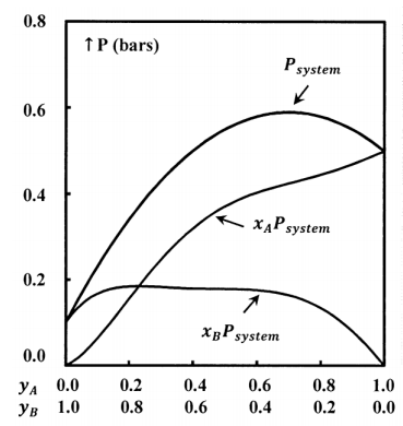
We determine the compositions of the gas and liquid phases by chemical analysis; for each system, we determine \(P\), \(x_A\), \(x_B\), \(y_A\), and \(y_B\). From these data we can develop empirical equations that express \(P\), \(x_A\), and \(x_B\)as functions of \(y_A\); that is, we have \(P=P\left(y_A\right)\), \(x_A=x_A\left(y_A\right)\), and \(x_B=x_B\left(y_A\right)\). Finally, we can find the value of the products \(x_AP\) and \(x_BP\). Figure 3 illustrates a possible function \(P=P\left(y_A\right)\) and the products \(x_AP\), and \(x_BP\), when the gas-phase mole fractions depend on \(y_A\) as shown in Figure 1.

Figure 3. Equilibrium pressures over a solution.

With the hypothetical ideal gas standard state as the standard state for \(A\) in the gas phase, we see in Section 14.11 that the chemical potential of \(A\) in the gas phase is

\[{\mu }_A\left(g,P,x_A,x_B\right)={\Delta }_fG^o\left(A,{HIG}^o\right)+RT{ \ln \left[\frac{x_AP}{P^o}\right]+RT\int^P_0{\left(\frac{{\overline{V}}_A\left(g\right)}{RT}-\frac{1}{P}\right)}\ }dP \nonumber \] (any gas; activity standard state is HIG\({}^{o}\))

where \({\overline{V}}_A\left(g\right)\) is the partial molar volume and \(x_A\) is the mole fraction of \(A\) in the gaseous mixture. The fugacity and activity of \(A\) in the gas phase are given by

\[{ \ln \left[{\tilde{a}}_A,P,x_A,x_B\right]\ }={ \ln \left[\frac{f_A\left(g,P,x_A,x_B\right)}{f_A\left({HIG}^o\right)}\right]\ }={ \ln \left[\frac{x_AP}{P^o}\right]+\int^P_0{\left(\frac{{\overline{V}}_A\left(g\right)}{RT}-\frac{1}{P}\right)}\ }dP \nonumber \]

and the standard state chemical potential is

\[{\mu }^o_A={\Delta }_fG^o\left(A,{HIG}^o\right) \nonumber \]

We want to express the chemical potential of \(A\) in the liquid solution using the properties of the solution. To do so, we introduce the chemical activity of component \(A\). We write \({\tilde{a}}_A\left(P,y_A,y_B\right)\) to represent the activity of \(A\) in a solution at pressure \(P\) and in which the composition is specified by the mole fractions \(y_A\) and \(y_B\). If it suits our purposes, we are free to choose a standard state for the activity of \(A\) in the liquid solution that is different from the standard state we choose for \(A\) in the gas phase. For reasons that become apparent below, it is often useful to choose the standard state for the activity of \(A\) in the liquid solution to be pure liquid \(A\) at its equilibrium vapor pressure, \(P^{\textrm{⦁}}_A\). We represent the chemical potential of \(A\) in this standard state by \({\widetilde{\mu }}^o_A\left(\ell ,P^{\textrm{⦁}}_A\right)\). Note that this state is not identical to the standard state for the pure liquid, for which the pressure is one bar and the chemical potential is \({\Delta }_fG^o\left(A,\ell \right)\). The chemical potential and the activity of A in the solution are related by

\[{\mu }_A\left(P,y_A,y_B\right)={\widetilde{\mu }}^o_A\left(\ell ,P^{\textrm{⦁}}_A\right)+RT{ \ln \left[{\tilde{a}}_A\left(P,y_A,y_B\right)\right]\ } \nonumber \] (any solution; activity standard state for \(A\) in solution is pure liquid \(A\) at its equilibrium vapor pressure)

Since the system is at equilibrium, we have

\[{\mu }_A\left(g,P,x_A,x_B\right)={\mu }_A\left(P,y_A,y_B\right) \nonumber \]

Equating our equations for these quantities, we find

\[{ \ln \left[{\tilde{a}}_A\left(P,y_A,y_B\right)\right]\ }=\frac{{\Delta }_fG^o\left(A,{HIG}^o\right)-{\widetilde{\mu }}^o_A\left(\ell ,P^{\textrm{⦁}}_A\right)}{RT}+{ \ln \left[\frac{x_AP}{P^o}\right]+\int^P_0{\left(\frac{{\overline{V}}_A\left(g\right)}{RT}-\frac{1}{P}\right)}\ }dP \nonumber \]

This equation gives the activity of \(A\) in a liquid solution whose state is specified by the liquid-phase mole fraction \(y_A\). In particular, it must give the activity of \(A\) in the “solution” for which \(y_A=1\) and \(y_B=0\); of course, this “solution” is pure liquid \(A\). At equilibrium with pure liquid \(A\), the gas phase contains pure gaseous \(A\); therefore, we have \(x_A=1\) and \(P=P^{\textrm{⦁}}_A\). The gas-phase partial molar volume is that for the pure gas, \({\overline{V}}^{\textrm{⦁}}_A\left(g\right)\). Moreover, this “solution” is the standard state for the activity of component \(A\), for which the activity of \(A\) is unity; that is,

\({\tilde{a}}_A\left(P,y_A,y_B\right)={\tilde{a}}_A\left(P^{\textrm{⦁}}_A,1,0\right)=1\). Making these substitutions into our equation for \({ \ln \left[{\tilde{a}}_A\left(P,y_A,y_B\right)\right]\ }\) and rearranging, we find

\[\frac{{\Delta }_fG^o\left(A,{HIG}^o\right)-{\widetilde{\mu }}^o_A\left(\ell ,P^{\textrm{⦁}}_A\right)}{RT}=-{ \ln \left[\frac{P^{\textrm{⦁}}_A}{P^o}\right]-\int^{P^{\textrm{⦁}}_A}_0{\left(\frac{{\overline{V}}^{\textrm{⦁}}_A\left(g\right)}{RT}-\frac{1}{P}\right)}\ }dP \nonumber \]

Substituting this result into our general equation for \( \ln \left[ \tilde{a}_A\left(P,y_A,y_B\right)\right]\) we find a completely general function for the activity of component \(A\).

\[ \ln \left[ \tilde{a}_A \left(P, y_A, y_B \right) \right] = \ln \left[ \frac{x_A P}{P^{\cdot}_A} \right] - \int_0^{P_A^{cdot}} \left( \frac{ \overline{V}_A^{\cdot} \left( g \right)}{RT} - \frac{1}{P} \right) dP + \int_)^P \left( \frac{ \overline{V}_A \left( g \right)}{RT} - \frac{1}{P} \right) dP \nonumber \]

(any solution; \(x_A\) is the mole fraction in the gas; the standard state for \(A\) in solution is the pure liquid at its equilibrium vapor pressure)

In such a system, the roles of solute and solvent are interchangeable. Interchanging the labels “\(A\)” and “B” gives an equation for the activity of component \(B\).

As circumstances warrant, several approximations can be applied to this result. When the partial molar volume of \(A\) in the gas, \({\overline{V}}_A\left(g\right)\), is not available, some approximation is required. Perhaps the least drastic approximation is that introduced in Section 14.11. We equate the unknown partial molar volume to the partial molar volume of the pure real gas at the same system pressure. Setting \({\overline{V}}_A\left(g\right)={\overline{V}}^{\textrm{⦁}}_A\left(g\right)\), we have

\[{ \ln \left[{\tilde{a}}_A\left(P,y_A,y_B\right)\right]\ }={ \ln \left[\frac{x_AP}{P^{\textrm{⦁}}_A}\right]+\int^P_{P^{\textrm{⦁}}_A}{\left(\frac{{\overline{V}}^{\textrm{⦁}}_A\left(g\right)}{RT}-\frac{1}{P}\right)}\ }dP \nonumber \]

Other approximations lead to greater simplifications. In the following sections, we discuss several. All of them assume that the components behave ideally in the gas phase. In this case, the integrals in our general equation for \({ \ln \left[{\tilde{a}}_A\left(\ P,y_A,y_B\right)\right]\ }\) vanish. Then,

\[{ \ln \left[{\tilde{a}}_A\left(P,y_A,y_B\right)\right]\ }={ \ln \left[\frac{x_AP}{P^{\textrm{⦁}}_A}\right]\ } \nonumber \]

(solution; \(x_A\) is the mole fraction in the ideal gas that is at equilibrium with the solution)

Our general result gives the activity of component \(A\) in solution using the mole fraction of its own vapor in the equilibrium system. When we have an empirical function, \(x_A=x_A\left(y_A\right)\), that relates the mole fraction in the gas to that in the solution, we can make this substitution and express the activity of \(A\) in the solution using its concentration in the solution. In the next several sections, we develop some basic methods for finding \(x_A=x_A\left(y_A\right)\).