16.11: Colligative Properties - Freezing-point Depression

The boiling point of a pure solvent, at a specified pressure, is the temperature at which the chemical potential of the pure solvent gas is equal to the chemical potential of the pure solvent liquid. The boiling point of a solution that contains a nonvolatile solute is the temperature at which the chemical potential of the pure solvent gas is equal to the chemical potential of the solvent in the solution. In the preceding section, we found that the boiling point of the solution is greater than the boiling point of the pure solvent. The temperature difference is the boiling-point elevation.

Similarly, the freezing point of a pure solvent, at a specified pressure, is the temperature at which the chemical potential of the pure-solid solvent is equal to the chemical potential of the pure-liquid solvent. The freezing point of a solution is the temperature at which the chemical potential of the pure-solid solvent is equal to the chemical potential of the solution-phase solvent. We find that the freezing point of the solution is less than the freezing point of the pure solvent. The temperature difference is the freezing-point depression.

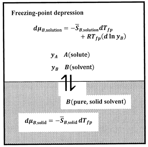
In the boiling-point elevation case, we assume that the pure solvent gas contains no solute. In the freezing-point depression case, we assume that the pure solvent solid contains no solute. We find the relationship between composition and freezing-point depression by an argument very similar to that for boiling-point elevation. The equilibrium state in the freezing-point depression experiment is described schematically in Figure 8.

Figure 8. Schematic description of freezing-point depression.

Since the equilibrium temperature decreases as the solute concentration increases, we can realize the equilibrium state experimentally by slowly cooling a solution of the specified composition. We determine the temperature at which the first, very small, crystal of solid solvent forms. Because the pure solvent freezes at a higher temperature than any solution, the first crystal formed is nearly pure solid solvent. Since this first crystal is very small, its formation does not change the composition of the solution significantly. Hence, the solution is in equilibrium with pure solid solvent at this temperature; we call this temperature the freezing point of the solution.

In practice, it is common to determine the melting point of a solid mixture rather than the freezing point of the liquid solution. The temperature of the solid mixture is increased slowly. As the mixture melts to form a homogeneous solution, the solute–solvent ratio in the melt approaches the ratio in which the mixture was prepared. When the last bit of solid melts, the composition of the solution is known from the manner of preparation. This last bit of solid melts at the highest temperature of any part of the mixture. It contains therefore the smallest proportion of solute. If this last bit of solid is in fact pure solvent, the temperature at which the last solid melts is the freezing point of the liquid solution. In the limit that the freezing-point and melting-point experiments are carried out reversibly, the state of the freezing-point system just after the first bit of solid freezes is the same as the state of the melting-point system just before the last bit of solid melts.

We again specify the composition of the solution by the mole fractions of \(A\) and\(\ B\). We let the solute be compound \(A\), and assume that its concentration is low. We let the solute concentration be \(y_A\), where \(y_A=1-y_B\), \(y_A\approx 0\) and \(y_B=1-y_A\approx 1\). The \(A\)–\(B\) solution is in equilibrium with pure solid \(B\). We want to find the temperature at which these phases are in equilibrium. At this temperature, \(\mu_{B,\mathrm{solution}}=\mu_{B,\mathrm{solid}}\), and hence \(d\mu_{B,\mathrm{solution}}=d\mu_{B,\mathrm{solid}}\) for any change that takes the system to a new equilibrium state.

We can analyze the freezing-point depression phenomenon for any fixed pressure at which pure-liquid \(B\) can be in equilibrium with pure-solid\(\ B\). Let us designate the fixed pressure as \(P^{\#}\) and the freezing-point temperature of pure-liquid B, at \(P^{\#}\), as \(T_F\). Our goal is to find the temperature at which a binary solution is in equilibrium with pure-solid \(B\) at the fixed pressure \(P^{\#}\). We let \(T_{fp}\) be the freezing-point temperature of the solution at \(P^{\#}\). We base our analysis on the assumption that \(A\) obeys Henry’s law.

We let the pure-solid solvent be the standard state for the solid solvent (see Section 15.5). Then, at every temperature, \(\mu_{B,\mathrm{solid}}={\widetilde\mu}^o_{B,\mathrm{solid}}\), and

\[\mu_{B,\mathrm{solid}}-{\widetilde\mu}^o_{B,\mathrm{solid}}=RT{ \ln {\tilde{a}}_{B,\mathrm{solid}}\ }=0 \nonumber \] At every temperature, \({\tilde{a}}_{B,\mathrm{solid}}=1\) so that \({\left({ \ln {\tilde{a}}_{B,\mathrm{solid}}\ }\right)}_{PT}=0\). The system pressure is constant at \(P^{\#}\), so \(dP=0\). In the general expression

\[d\mu_{B,\mathrm{solid}}=\overline{V}_{B,\mathrm{solid}}dP-\overline{S}_{B,\mathrm{solid}}dT+RT{\left(d{ \ln {\tilde{a}}_{B,\mathrm{solid}}\ }\right)}_{PT} \nonumber \]

only the term in \(dT\) is non-zero. Recognizing that \(dT\) is the change in the freezing-point temperature at \(P^{\#}\), for some change in the chemical potential of pure solid \(B\), we have

\[d\mu_{B,\mathrm{solid}}=-\overline{S}^{\textrm{⦁}}_{B,\mathrm{solid}}\ dT_{fp} \nonumber \]

We let the pure-liquid solvent at its equilibrium vapor pressure be the standard state for the solution-phase solvent (see Section 16.2). We designate this equilibrium vapor pressure as \(P^{\textrm{⦁}}_B\left(T_{fp}\right)\). Now, since we ultimately find \(T_{fp}<t_f\)>, the pure liquid freezes spontaneously at \(T_{fp}\). The standard state for the liquid solvent is therefore a hypothetical state; it is a pure, super-cooled liquid. The properties of this hypothetical liquid can be estimated from our theory; however, except possibly in unusual circumstances, they cannot be measured directly. Since we assume that the solute obeys Henry’s law, we have from Section 16.8 that \(d{ \ln {\tilde{a}}_{B,\mathrm{solution}}=d{ \ln y_B\ }\ }\). Thus, while the activity of the pure-solid solvent is constant, the activity of the solvent in the solution varies with the solute concentration. We have

\[d\mu_{B,\mathrm{solution}}=-\overline{S}_{B,\mathrm{solution}}\ dT_{fp}+RT_{fp}{\left(d{ \ln y_B\ }\right)}_{PT} \nonumber \]

Using \(d{ \ln y_B\ }\approx -dy_A\), the relationship \(d\mu_{B,\mathrm{solution}}=d\mu_{B,\mathrm{solid}}\) becomes

\[-\overline{S}_{B,\mathrm{solution}}\ dT_{fp}-RT_{fp}dy_A=-\overline{S}^{\textrm{⦁}}_{B,\mathrm{solid}}\ dT_{fp} \nonumber \]

or

\[dy_A=-\left(\frac{\overline{S}_{B,\mathrm{solution}}-\overline{S}^{\textrm{⦁}}_{B,\mathrm{solid}}}RT_{fp}\right)dT_{fp} \nonumber \]

We consider systems in which the freezing point of the solution, \(T_{fp}\), is little different from the freezing point of the pure solvent, \(T_F\). Then, \(T_F\approx T_{fp}\), and \({T_{fp}}/{T_F}\approx 1\). We let \(\left|\Delta T\right|=T_F-T_{fp}\), where \(\left|\Delta T\right|\ll T_F\). Since the solution is almost pure \(B\), the partial molar entropy of \(B\) in the solution is approximately that of pure liquid \(B\). Consequently, the partial molar entropy difference is, to a good approximation, just the entropy of fusion of the pure solvent, at equilibrium, at the freezing point for the specified system pressure. That is,

\[{\left(\overline{S}_{B,\mathrm{solution}}-\overline{S}^{\textrm{⦁}}_{B,\mathrm{solid}}\right)}_{P^{\#},T_{fp}}\approx {\left(\overline{S}^{\textrm{⦁}}_{B,\mathrm{liquid}}-\overline{S}^{\textrm{⦁}}_{B,\mathrm{solid}}\right)}_{P^{\#},T_F}=\Delta_{\mathrm{fus}}S_B={\Delta_{\mathrm{fus}}H_B}/{T_F} \nonumber \]

so that \[dy_A=-\left(\frac{\Delta_{\mathrm{fus}}H_B}{RT_{fp}T_F}\right)dT_{fp} \nonumber \]

At \(P^{\#}\) and \(T_F\), \(\Delta_{\mathrm{fus}}H_B\) is a constant. In the solution, the solute mole fraction is \(y_A\); in the pure solid solvent, it is zero. Integrating between the limits \(\left(0,T_F\right)\) and \(\left(y_A,T_{fp}\right)\), we have

\[\int^{y_A}_0{dy_A}=-\frac{\Delta_{\mathrm{fus}}H_B}{RT_F}\int^{T_{fp}}_{T_F}{\frac{dT_{fp}}{T_{fp}}} \nonumber \] and \[y_A=-\frac{\Delta_{\mathrm{fus}}H_B}{RT_F}{ \ln \frac{T_{fp}}{T_F}\ } \nonumber \]

Introducing \({ \ln x\approx x-1\ }\), we have \[y_A=-\frac{\Delta_{\mathrm{fus}}H_B}{RT_F}\left(\frac{T_{fp}}{T_F}-1\right)=\frac{\Delta_{\mathrm{fus}}H_B}{RT^2_F}\Delta T \nonumber \] Solving for \(\Delta T\), \[\Delta T=\left(\frac{RT^2_F}{\Delta_{\mathrm{fus}}H_B}\right)y_A \nonumber \]

The fusion process is endothermic, and \(\Delta_{\mathrm{fus}}H_B>0\). Therefore, we find \(\Delta T=T_F-T_{fp}>0\); that is, the addition of a solute decreases the freezing point of a liquid. The depression of the freezing point is proportional to the solute concentration.

Since measurement of \(\Delta T\) enables us to find \(y_A\), freezing-point depression—like boiling point elevation—enables us to determine the molar mass of a solute. In our discussion of boiling-point elevation, we noted that it is often convenient to express the concentration of a dilute solute in units of molality rather than mole fraction. This applies also to freezing-point depression. Likewise, for practical applications, we usually find the freezing-point depression constant by measuring the depression of the freezing point of a solution of known composition.