16.12: Colligative Properties - Osmotic Pressure

The phenomena of boiling-point elevation and freezing-point depression involve relationships between composition and equilibrium temperature—at constant system pressure. We turn now to a phenomenon, osmotic pressure, which involves a relationship between composition and equilibrium pressure—at constant system temperature.

To analyze boiling-point elevation, we equate the chemical potential of the solvent in two subsystems, a solution and the gas phase above it. To analyze freezing-point depression, we equate the chemical potential of the solvent in solution and solid subsystems. Similarly, to analyze osmotic pressure, we equate the chemical potential of the pure solvent—at one pressure—to the chemical potential of the solvent in a solution—at a second pressure. We find that equilibrium can be obtained only when the pressure in the solution subsystem exceeds the pressure in the solvent subsystem. The difference between these two pressures is the osmotic pressure.

In the boiling-point elevation and freezing-point depression phenomena, the subsystems are separated by a phase boundary. In the osmotic pressure phenomenon, a pure solvent phase is separated from a solution phase by a semi-permeable membrane. A semi-permeable membrane allows free passage to solvent molecules; however, solute molecules cannot pass through it. In practice, the semi-permeable membrane is a material that is penetrated by pores, or channels, whose cross-sectional dimensions are nearly as small as typical solvent molecules. Solvent molecules can diffuse through these pores and pass from one side of the membrane to the other. With such a membrane, we can satisfy the osmotic pressure conditions by choosing a solute whose molecules are larger than the pore diameters, because large molecules will be unable to pass through the pores. In practice, the solute in osmotic pressure experiments is typically a polymer or a biologically derived molecule of high molecular weight. Osmotic pressure measurements have been an important source of data on the molar masses of such substances.

Figure 9. Schematic description of osmotic pressure.

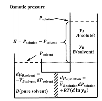
The osmotic pressure experiment is described schematically in Figure 9. The semi-permeable membrane must be sufficiently robust to support the pressure drop between the two subsystems. At constant pressure, mixing of the two subsystems is a spontaneous process. Were we to remove the membrane and the pressure drop that it supports, the subsystems would mix to form a single, more dilute solution. We see therefore that there is a tendency for net migration of solvent molecules from the solvent side of the membrane to the solution side. We can oppose this tendency by applying additional pressure on the solution side. Evidently, for any given solution composition, there will be an applied pressure at which the subsystems are in equilibrium with one another.

We let the pure-liquid solvent at its equilibrium vapor pressure be the standard state for both the pure-liquid and the solution-phase solvent (see Section 16.2). For the two subsystems to be in equilibrium, we must have \({\mu }_{B,\mathrm{soluton}}={\mu }_{B,\mathrm{solvent}}\). For any change that takes one equilibrium state to another, we have \(d{\mu }_{B,\mathrm{soluton}}=d{\mu }_{B,\mathrm{solvent}}\). Since the pure solvent subsystem contains only \(B\), we have \({\tilde{a}}_{B,\mathrm{so}\mathrm{lvent}}=\mathrm{constant}\) so that \(d{ \ln {\tilde{a}}_{B,\mathrm{sol}\mathrm{vent}}\ }=0\). Since the temperature is constant, we have \(dT=0\). For the solvent subsystem, the general expression for\(\ d{\mu }_{B,\mathrm{solvent}}\) reduces to

\[d{\mu }_{B,\mathrm{solvent}}={\overline{V}}^{\textrm{⦁}}_{B,\mathrm{solvent}}dP_{\mathrm{solvent}} \nonumber \]

For the solution subsystem, \(dT=0\). Assuming the solvent in the solution obeys Raoult’s law, we have \({\tilde{a}}_{B,\mathrm{sol}\mathrm{ution}}=y_B\). The general equation for \(d{\mu }_{B,\mathrm{soluton}}\) reduces to

\[d{\mu }_{B,\mathrm{soluton}}=\overline{V}_{B,\mathrm{solution}}dP_{\mathrm{solution}}+RT\left(d{ \ln y_B\ }\right) \nonumber \]

Using \(d{ \ln y_B\ }\approx -dy_A\), the relationship \(d{\mu }_{B,\text{solution}}=d{\mu }_{B,\mathrm{solvent}}\) becomes

\[{\overline{V}}_{B,\mathrm{solution}}dP_{\mathrm{solution}}-RTdy_A={\overline{V}}^{\textrm{⦁}}_{B,\mathrm{solvent}}dP_{\mathrm{solvent}} \nonumber \]

The molar volume of a liquid is nearly independent of the system pressure. Because the solution is nearly pure solvent, the molar volume of \(B\) in the solution is approximately equal to the molar volume of pure solvent \(B\). Letting \(\overline{V}_{B,\mathrm{solution}}=\overline{V}^{\textrm{⦁}}_{B,\mathrm{solvent}}={\overline{V}}^{\textrm{⦁}}_B\), this becomes

\[dy_A=\left(\frac{\overline{V}^{\textrm{⦁}}_B}{RT}\right)\left(dP_{\mathrm{solution}}-dP_{\mathrm{solvent}}\right)=\left(\frac{\overline{V}^{\textrm{⦁}}_B}{RT}\right)\ d\left(P_{\mathrm{solution}}-P_{\mathrm{solvent}}\right) \nonumber \]

This pressure difference is the osmotic pressure; it is often represented by the Greek alphabet capital pi: \(\mathit{\Pi}=P_{\mathrm{solution}}-P_{\mathrm{solvent}}\). The osmotic pressure of the pure solvent must be zero; that is, \(\mathit{\Pi}=0\) when \(y_A=0\). Integrating between the limits \(\left(0,0\right)\) and \(\left(y_A,\mathit{\Pi}\right)\), we have

\[\int^{y_A}_0{dy_A}=\frac{\overline{V}^{\textrm{⦁}}_B}{RT}\int^{\mathit{\Pi}}_0{d\mathit{\Pi}} \nonumber \]

and

\[y_A=\frac{\overline{V}^{\textrm{⦁}}_B\mathit{\Pi}}{RT} \nonumber \]

or

\[{\mathit{\Pi}\overline{V}}^{\textrm{⦁}}_B=y_ART \nonumber \]

From this equation, we see that the osmotic pressure must be positive; that is, at equilibrium, the pressure on the solution must be greater than the pressure on the solvent: \(\mathit{\Pi}=P_{\mathrm{solution}}-P_{\mathrm{solvent}}>0\).

The osmotic pressure equation can be put into an easily remembered form. For \(n_A\ll n_B\), \(y_A={n_A}/{\left(n_A+n_B\right)\approx {n_A}/{n_B}}\). With this substitution, \(\mathit{\Pi}\left(n_B{\overline{V}}^{\textrm{⦁}}_B\right)=n_ART\), but since \({\overline{V}}^{\textrm{⦁}}_B\) is the molar volume of pure \(B\), \(V=n_B{\overline{V}}^{\textrm{⦁}}_B\) is just the volume of the solvent and essentially the same as the volume of the solution. The osmotic pressure equation has the same form as the ideal gas equation:

\[\mathit{\Pi}\left(n_B{\overline{V}}^{\textrm{⦁}}_B\right)=\mathit{\Pi}\ V=n_ART \nonumber \]