14.14: Dependence of Activity on Temperature- Relative Partial Molar Enthalpies

Having found the activity of a component at one temperature, we want to be able to find it at a second temperature. The equation developed in Section 14.13 does not provide a practical way to find the temperature dependence of \({\tilde{a}}_A\) or \({ \ln {\tilde{a}}_A\ }\). We can obtain a useful equation by rearranging the defining equation, taking the partial derivative of \({ \ln {\tilde{a}}_A\ }\) with respect to temperature, and making use of the Gibbs-Helmholtz equation:

\[\begin{aligned} \left(\frac{\partial \ln \tilde{a}_A}{\partial T} \right)_P & =\left[\frac{\partial }{\partial T}\left(\frac{{\mu }_A}{RT}-\frac{ \widetilde{\mu }^o_A}{RT}\right)\right]_P \\ ~ & =\frac{1}{R}\left[ \left(\frac{\partial \left({\mu }_A/T \right)}{\partial T}\right)_P- \left(\frac{\partial \left( \widetilde{\mu }^o_A/T\right)}{\partial T}\right)_P\right] \\ ~ & =-\frac{\overline{H}_A}{RT^2}+\frac{\tilde{H}^o_A}{RT^2} \end{aligned} \nonumber \]

\({\overline{H}}_A\) is the partial molar enthalpy of component \(A\) as it is present in the system. \({\tilde{H}}^o_A\) is the partial molar enthalpy of component \(A\) in its activity standard state. Since this standard state need not correspond to any real system, \({\tilde{H}}^o_A\) can be the partial molar enthalpy of the substance in a hypothetical state.

In general, it is not possible to find \(-\left({\overline{H}}_A-{\tilde{H}}^o_A\right)\) by experimental measurement of the heat exchanged in a single-step process in which \(A\) passes from its state in the system of interest to its activity standard state. Instead, we devise a multi-step cycle in which we can determine the enthalpy change for each step. This cycle includes yet another state of substance \(A\), which we call the reference state and whose molar enthalpy we designate as \({\overline{H}}^{ref}_A\). We devise this cycle to find two enthalpy changes. One is the enthalpy change that occurs when one mole of \(A\) passes from the system of interest to the reference state; this enthalpy change is represented by the difference \(-\left({\overline{H}}_A-{\overline{H}}^{ref}_A\right)\). The other is the enthalpy change that occurs when one mole of A passes from the activity standard state to the reference state. This enthalpy change is represented by the difference \(-\left({\tilde{H}}^o_A-{\overline{H}}^{ref}_A\right)\). The enthalpy change we seek is the difference between these two differences:

\[-\left({\overline{H}}_A-{\tilde{H}}^o_A\right)=-\left({\overline{H}}_A-{\overline{H}}^{ref}_A\right)+\left({\tilde{H}}^o_A-{\overline{H}}^{ref}_A\right) \nonumber \]

Because we explicitly choose the reference state so that these differences are experimentally measurable, it is useful to introduce still more terminology. We define the relative partial molar enthalpy of substance \(A\), \({\overline{L}}_A\), as the difference between the partial molar enthalpy of \(A\) in the state of interest, \({\overline{H}}_A\), and the partial molar enthalpy of A in the reference state, \({\overline{H}}^{ref}_A\); that is, \({\overline{L}}_A={\overline{H}}_A-{\overline{H}}^{ref}_A\) and \({\tilde{L}}^o_A={\tilde{H}}^o_A-{\overline{H}}^{ref}_A\) where \({\tilde{L}}^o_A\) is the relative partial molar enthalpy of substance \(A\) in the activity standard state. Clearly, the values of \({\overline{L}}_A\) and \({\tilde{L}}^o_A\) depend on the choice of reference state. We choose the reference state so that \({\overline{L}}_A\) and \({\tilde{L}}^o_A\) can be measured directly. The quantity that we must evaluate experimentally in order to find \({\left({\partial { \ln {\tilde{a}}_A\ }}/{\partial T}\right)}_P\) becomes

\[-\left({\overline{H}}_A-{\tilde{H}}^o_A\right)=-\left({\overline{L}}_A-{\tilde{L}}^o_A\right) \nonumber \]

To see how these ideas and definitions can be given practical effect, let us consider a binary solution that comprises a relatively low concentration of solute, \(A\), in a solvent, \(B\), at a fixed pressure, normally one bar. We suppose that pure \(A\) is a solid and pure \(B\) is a liquid in the temperature range of interest. We need to choose an activity standard state and an enthalpy reference state for each substance. The most generally useful choices use the concept of an infinitely dilute solution. In an infinitely dilute solution, \(A\) molecules are dispersed so completely that they can interact only with \(B\) molecules. Consequently, the energy of the \(A\) molecules cannot change if additional pure solvent (initially at the same temperature and pressure) is added. Operationally then, we can recognize an infinitely dilute solution by mixing it with additional pure solvent; if no heat must be exchanged with the surroundings in order to keep the temperature constant, the original solution is infinitely dilute.

For the solvent, the concept of an infinitely dilute solution gives rise to the following choices, which are shown schematically in Figure 3:

Figure 3. Cycles relating the molar enthalpy of a solvent to its molar enthalpies in the pure liquid, in an activity standard state, and in an enthalpy standard state.

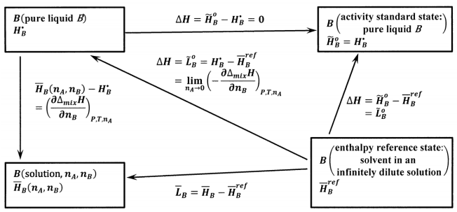
For the activity standard state of the solvent, \(B\), we choose pure liquid \(B\). Then, the activity of pure liquid \(B\) is unity at any temperature. Letting \({\tilde{H}}^o_B\) be the partial molar enthalpy of \(B\) in the activity standard state and \(H^{\textrm{⦁}}_B\) be the molar enthalpy of pure liquid \(B\), we have \({\tilde{H}}^o_B=H^{\textrm{⦁}}_B\).

For the enthalpy reference state of the solvent, we choose \(B\) in an infinitely dilute solution. We represent the partial molar enthalpy of \(B\) in this infinitely dilute solution by \({\overline{H}}^{ref}_B\).

For the solute, the infinitely dilute solution involves the following choices, which are shown schematically in Figure 4:

For the activity standard state of the solute, we choose the hypothetical solution in which the concentration of \(A\) is one molal, and the activity of \(A\) is unity, but all of the effects of intermolecular interactions are the same as they are in an infinitely dilute solution. We represent the partial molar enthalpy of \(A\) in the activity standard state by \({\tilde{H}}^o_A\).

For the enthalpy reference state of the solute, we choose the infinitely dilute solution and designate the partial molar enthalpy of \(A\) in this reference state by \({\overline{H}}^{ref}_A\). Since all of the intermolecular interactions are the same in the enthalpy reference state as they are in the activity standard state, there can be no energy change when one mole of \(A\) goes from one of these states to the other. It follows that \({\tilde{H}}^o_A={\overline{H}}^{ref}_A\).

It follows from these choices that the relative partial molar enthalpies of \(A\) and \(B\) in their activity standard states are \({\tilde{L}}^o_A={\tilde{H}}^o_A-{\overline{H}}^{ref}_A=0\) and

\[{\tilde{L}}^o_B={\tilde{H}}^o_B-{\overline{H}}^{ref}_B={\mathop{\mathrm{lim}}_{n_A\to 0} {\left(-\frac{\partial {\Delta }_{mix}H}{\partial n_B}\right)}_{P,T,n_A}\ } \nonumber \]

The relevant process for which we can measure an enthalpy change is the isothermal mixing of \(n_A\) moles of pure solid \(A\) with \(n_B\) moles of pure liquid \(B\) to form a solution:

\[{n_AA\left(\mathrm{pure\ solid}\right)+n}_BB\left(\mathrm{pure\ liquid}\right) \begin{array}{c} {\Delta }_{mix}H \\ \to \\ \end{array} {A}/{B\left(\mathrm{solution},\ n_A,n_B\right)} \nonumber \]

Letting the enthalpy of mixing be \({\Delta }_{mix}H\) and the enthalpy of the resulting solution be \(H\), we have

\[H={\Delta }_{mix}H+n_AH^{\textrm{⦁}}_A+n_BH^{\textrm{⦁}}_B \nonumber \]

Then

\[{\overline{H}}_A={\left(\frac{\partial H}{\partial n_A}\right)}_{PT}={\left(\frac{\partial {\Delta }_{mix}H}{\partial n_A}\right)}_{PT}+H^{\textrm{⦁}}_A \nonumber \]

and

\[{\overline{H}}_B={\left(\frac{\partial H}{\partial n_B}\right)}_{PT}={\left(\frac{\partial {\Delta }_{mix}H}{\partial n_B}\right)}_{PT}+H^{\textrm{⦁}}_B \nonumber \] where, of course, \(H\), \({\Delta }_{mix}H\), \({\overline{H}}_A\), and \({\overline{H}}_B\) are all functions of \(n_A\) and \(n_B\). The partial molar enthalpies in the reference states are the limiting values of \({\overline{H}}_A\) and \({\overline{H}}_B\) as \(n_A\to 0\). That is,

\[{\overline{H}}^{ref}_A={\mathop{\mathrm{lim}}_{n_A\to 0} {\left(\frac{\partial {\Delta }_{mix}H}{\partial n_A}\right)}_{P,T,n_B}\ }+H^{\textrm{⦁}}_A \nonumber \] and \[{\overline{H}}^{ref}_B={\mathop{\mathrm{lim}}_{n_B\to 0} {\left(\frac{\partial {\Delta }_{mix}H}{\partial n_B}\right)}_{P,T,n_A}\ }+H^{\textrm{⦁}}_B \nonumber \]

When we base the enthalpy reference states on the infinitely dilute solution, we find for the solute

\[-\left({\overline{H}}_A-{\tilde{H}}^o_A\right)=-\left({\overline{H}}_A-{\overline{H}}^{ref}_A\right)+\left({\tilde{H}}^o_A-{\overline{H}}^{ref}_A\right) \nonumber \] \[=-\left({\overline{L}}_A-{\tilde{L}}^o_A\right)=-{\overline{L}}_A=-{\left(\frac{\partial {\Delta }_{mix}H}{\partial n_A}\right)}_{P,T,n_B}+{\mathop{\mathrm{lim}}_{n_A\to 0} {\left(\frac{\partial {\Delta }_{mix}H}{\partial n_A}\right)}_{P,T,n_B}\ } \nonumber \]

and for the solvent

\[-\left({\overline{H}}_B-{\tilde{H}}^o_B\right)=-\left({\overline{H}}_B-{\overline{H}}^{ref}_B\right)+\left({\tilde{H}}^o_B-{\overline{H}}^{ref}_B\right)=-\left({\overline{L}}_B-{\tilde{L}}^o_B\right)=-{\left(\frac{\partial {\Delta }_{mix}H}{\partial n_B}\right)}_{P,T,n_A} \nonumber \]

The temperature dependence of the activities becomes

\[{\left(\frac{\partial { \ln {\tilde{a}}_A\ }}{\partial T}\right)}_P=\frac{1}{RT^2}\left[-{\left(\frac{\partial {\Delta }_{mix}H}{\partial n_A}\right)}_{P,T,n_B}+{\mathop{\mathrm{lim}}_{n_A\to 0} {\left(\frac{\partial {\Delta }_{mix}H}{\partial n_A}\right)}_{P,T,n_B}\ }\right] \nonumber \]

and \[{\left(\frac{\partial { \ln {\tilde{a}}_B\ }}{\partial T}\right)}_P=-\frac{1}{RT^2}{\left(\frac{\partial {\Delta }_{mix}H}{\partial n_B}\right)}_{P,T,n_A} \nonumber \]

To a good first approximation, we can measure \({\Delta }_{mix}H\) as a function of composition at a single temperature, determine \({\overline{L}}_A\) and \({\overline{L}}_B-{\tilde{L}}^o_B\) at that temperature, and assume that these values are independent of temperature. For a more exact treatment, we can measure \({\Delta }_{mix}H\) as a function of composition at several temperatures and find \({\overline{L}}_A\) and \({\overline{L}}_B-{\tilde{L}}^o_B\) as functions of temperature. It proves to be useful to define the relative partial molar heat capacity of \(A\), to which we give the symbol, \({\overline{J}}_A\), as the temperature derivative of \({\overline{L}}_A\):

\[{\overline{J}}_A={\left(\frac{\partial {\overline{L}}_A}{\partial T}\right)}_P \nonumber \]

To illustrate the use of these ideas, let us suppose that we measure the enthalpy of mixing of solute \(A\) in 1 kg water (solvent \(B\)). We make this measurement for several quantities of \(A\) at each of several temperatures between 273.15 K and 293.15 K. For each experiment in this series, \(n_B\) is 55.51 mole and \(n_A\) is equal to the molality of \(A\), \(\underline{m}\), in the solution. We fit the experimental data to empirical equations. Let us suppose that the enthalpy of mixing data at any given temperature are described adequately by the equation \({\Delta }_{mix}H={\alpha }_1\underline{m}+{\alpha }_2{\underline{m}}^2\) and that \({\alpha }_1\) and \({\alpha }_2\) depend linearly on \(T\) according to

\[{\alpha }_1={\beta }_{11}+{\beta }_{12}\left(T-273.15\right) \nonumber \] and

\[{\alpha }_2={\beta }_{21}+{\beta }_{22}\left(T-273.15\right) \nonumber \]

Then

\[{\left(\frac{\partial {\Delta }_{mix}H}{\partial n_A}\right)}_{P,T,n_B}={\left(\frac{\partial {\Delta }_{mix}H}{\partial \underline{m}}\right)}_{P,T,n_B}={\alpha }_1+2{\alpha }_2\underline{m} \nonumber \]

and

\[{\mathop{\mathrm{lim}}_{n_A\to 0} {\left(\frac{\partial {\Delta }_{mix}H}{\partial n_A}\right)}_{P,T,n_B}\ }={\alpha }_1 \nonumber \]

so that

\[{\overline{L}}_A={\left(\frac{\partial {\Delta }_{mix}H}{\partial n_A}\right)}_{P,T,n_B}-{\mathop{\mathrm{lim}}_{n_A\to 0} {\left(\frac{\partial {\Delta }_{mix}H}{\partial n_A}\right)}_{P,T,n_B}\ }=2{\alpha }_2\underline{m} \nonumber \]

and

\[\left(\frac{\partial \ln \tilde{a}_A}{\partial T}\right)_P=-\frac{\overline{L}_A}{RT^2}=-\frac{2{\alpha }_2\underline{m}}{RT^2} \nonumber \]

and

\[{\overline{J}}_A={\left(\frac{\partial {\overline{L}}_A}{\partial T}\right)}_P=2\underline{m}{\left(\frac{\partial {\alpha }_2}{\partial T}\right)}_P=2\underline{m}{\beta }_{22} \nonumber \]

In the experiments of this illustrative example, \(n_B\) is constant. This might make it seem that we would have to do an additional set of experiments, a set in which \(n_B\) is varied, in order to find \({\overline{L}}_B\), \({\left({\partial { \ln {\tilde{a}}_B\ }}/{\partial T}\right)}_P\), and \({\overline{J}}_B\). However, this is not the case. Since \({\overline{L}}_A\) and \({\overline{L}}_B\) are partial molar quantities, we have

\[n_Ad{\overline{L}}_A+n_Bd{\overline{L}}_B=0 \nonumber \] so that \[d{\overline{L}}_B=-\left(\frac{n_A}{n_B}\right)d{\overline{L}}_A \nonumber \]

and we can find \({\overline{L}}_B\) from

\[\overline{L}_B\left(\underline{m}\right)-\overline{L}_B\left(0\right)=\overline{L}_B\left(\underline{m}\right)=\int^{\underline{m}}_0 -\left(\frac{2\underline{m}{\alpha }_2}{55.51}\right)d\underline{m}=-\frac{\underline{m}^2{\alpha }_2}{55.51} \nonumber \]

and

\[\overline{J}_B= \left(\frac{\partial \overline{L}_B}{\partial T}\right)_P=-\frac{\underline{m}^2}{55.51} \left(\frac{\partial {\alpha }_2}{\partial T} \right)_{P,n_A}=-\frac{\underline{m}^2{\beta }_{22}}{55.51} \nonumber \]