Pulse Sequences
- Page ID
- 8023
\( \newcommand{\vecs}[1]{\overset { \scriptstyle \rightharpoonup} {\mathbf{#1}} } \)
\( \newcommand{\vecd}[1]{\overset{-\!-\!\rightharpoonup}{\vphantom{a}\smash {#1}}} \)
\( \newcommand{\dsum}{\displaystyle\sum\limits} \)
\( \newcommand{\dint}{\displaystyle\int\limits} \)
\( \newcommand{\dlim}{\displaystyle\lim\limits} \)
\( \newcommand{\id}{\mathrm{id}}\) \( \newcommand{\Span}{\mathrm{span}}\)
( \newcommand{\kernel}{\mathrm{null}\,}\) \( \newcommand{\range}{\mathrm{range}\,}\)
\( \newcommand{\RealPart}{\mathrm{Re}}\) \( \newcommand{\ImaginaryPart}{\mathrm{Im}}\)
\( \newcommand{\Argument}{\mathrm{Arg}}\) \( \newcommand{\norm}[1]{\| #1 \|}\)
\( \newcommand{\inner}[2]{\langle #1, #2 \rangle}\)
\( \newcommand{\Span}{\mathrm{span}}\)
\( \newcommand{\id}{\mathrm{id}}\)
\( \newcommand{\Span}{\mathrm{span}}\)
\( \newcommand{\kernel}{\mathrm{null}\,}\)
\( \newcommand{\range}{\mathrm{range}\,}\)
\( \newcommand{\RealPart}{\mathrm{Re}}\)
\( \newcommand{\ImaginaryPart}{\mathrm{Im}}\)
\( \newcommand{\Argument}{\mathrm{Arg}}\)
\( \newcommand{\norm}[1]{\| #1 \|}\)
\( \newcommand{\inner}[2]{\langle #1, #2 \rangle}\)
\( \newcommand{\Span}{\mathrm{span}}\) \( \newcommand{\AA}{\unicode[.8,0]{x212B}}\)
\( \newcommand{\vectorA}[1]{\vec{#1}} % arrow\)
\( \newcommand{\vectorAt}[1]{\vec{\text{#1}}} % arrow\)
\( \newcommand{\vectorB}[1]{\overset { \scriptstyle \rightharpoonup} {\mathbf{#1}} } \)
\( \newcommand{\vectorC}[1]{\textbf{#1}} \)
\( \newcommand{\vectorD}[1]{\overrightarrow{#1}} \)
\( \newcommand{\vectorDt}[1]{\overrightarrow{\text{#1}}} \)
\( \newcommand{\vectE}[1]{\overset{-\!-\!\rightharpoonup}{\vphantom{a}\smash{\mathbf {#1}}}} \)
\( \newcommand{\vecs}[1]{\overset { \scriptstyle \rightharpoonup} {\mathbf{#1}} } \)
\(\newcommand{\longvect}{\overrightarrow}\)
\( \newcommand{\vecd}[1]{\overset{-\!-\!\rightharpoonup}{\vphantom{a}\smash {#1}}} \)
\(\newcommand{\avec}{\mathbf a}\) \(\newcommand{\bvec}{\mathbf b}\) \(\newcommand{\cvec}{\mathbf c}\) \(\newcommand{\dvec}{\mathbf d}\) \(\newcommand{\dtil}{\widetilde{\mathbf d}}\) \(\newcommand{\evec}{\mathbf e}\) \(\newcommand{\fvec}{\mathbf f}\) \(\newcommand{\nvec}{\mathbf n}\) \(\newcommand{\pvec}{\mathbf p}\) \(\newcommand{\qvec}{\mathbf q}\) \(\newcommand{\svec}{\mathbf s}\) \(\newcommand{\tvec}{\mathbf t}\) \(\newcommand{\uvec}{\mathbf u}\) \(\newcommand{\vvec}{\mathbf v}\) \(\newcommand{\wvec}{\mathbf w}\) \(\newcommand{\xvec}{\mathbf x}\) \(\newcommand{\yvec}{\mathbf y}\) \(\newcommand{\zvec}{\mathbf z}\) \(\newcommand{\rvec}{\mathbf r}\) \(\newcommand{\mvec}{\mathbf m}\) \(\newcommand{\zerovec}{\mathbf 0}\) \(\newcommand{\onevec}{\mathbf 1}\) \(\newcommand{\real}{\mathbb R}\) \(\newcommand{\twovec}[2]{\left[\begin{array}{r}#1 \\ #2 \end{array}\right]}\) \(\newcommand{\ctwovec}[2]{\left[\begin{array}{c}#1 \\ #2 \end{array}\right]}\) \(\newcommand{\threevec}[3]{\left[\begin{array}{r}#1 \\ #2 \\ #3 \end{array}\right]}\) \(\newcommand{\cthreevec}[3]{\left[\begin{array}{c}#1 \\ #2 \\ #3 \end{array}\right]}\) \(\newcommand{\fourvec}[4]{\left[\begin{array}{r}#1 \\ #2 \\ #3 \\ #4 \end{array}\right]}\) \(\newcommand{\cfourvec}[4]{\left[\begin{array}{c}#1 \\ #2 \\ #3 \\ #4 \end{array}\right]}\) \(\newcommand{\fivevec}[5]{\left[\begin{array}{r}#1 \\ #2 \\ #3 \\ #4 \\ #5 \\ \end{array}\right]}\) \(\newcommand{\cfivevec}[5]{\left[\begin{array}{c}#1 \\ #2 \\ #3 \\ #4 \\ #5 \\ \end{array}\right]}\) \(\newcommand{\mattwo}[4]{\left[\begin{array}{rr}#1 \amp #2 \\ #3 \amp #4 \\ \end{array}\right]}\) \(\newcommand{\laspan}[1]{\text{Span}\{#1\}}\) \(\newcommand{\bcal}{\cal B}\) \(\newcommand{\ccal}{\cal C}\) \(\newcommand{\scal}{\cal S}\) \(\newcommand{\wcal}{\cal W}\) \(\newcommand{\ecal}{\cal E}\) \(\newcommand{\coords}[2]{\left\{#1\right\}_{#2}}\) \(\newcommand{\gray}[1]{\color{gray}{#1}}\) \(\newcommand{\lgray}[1]{\color{lightgray}{#1}}\) \(\newcommand{\rank}{\operatorname{rank}}\) \(\newcommand{\row}{\text{Row}}\) \(\newcommand{\col}{\text{Col}}\) \(\renewcommand{\row}{\text{Row}}\) \(\newcommand{\nul}{\text{Nul}}\) \(\newcommand{\var}{\text{Var}}\) \(\newcommand{\corr}{\text{corr}}\) \(\newcommand{\len}[1]{\left|#1\right|}\) \(\newcommand{\bbar}{\overline{\bvec}}\) \(\newcommand{\bhat}{\widehat{\bvec}}\) \(\newcommand{\bperp}{\bvec^\perp}\) \(\newcommand{\xhat}{\widehat{\xvec}}\) \(\newcommand{\vhat}{\widehat{\vvec}}\) \(\newcommand{\uhat}{\widehat{\uvec}}\) \(\newcommand{\what}{\widehat{\wvec}}\) \(\newcommand{\Sighat}{\widehat{\Sigma}}\) \(\newcommand{\lt}{<}\) \(\newcommand{\gt}{>}\) \(\newcommand{\amp}{&}\) \(\definecolor{fillinmathshade}{gray}{0.9}\)A pulse sequence is a succinct visual representation of the pulses and delays used in a certain NMR experiment. Depending on the experiment there may be hundreds of pulses! This page is dedicated to understanding what a pulse sequence is and how to understand the pictorial representations, as well as terms commonly used to describe parts of pulse sequences.
How to Read and Understand a Pulse Sequence
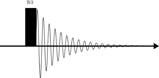
The most basic pulse sequence is a single pulse followed by detection of the signal. This is shown in figure 1. The pulse is represented by the large black bar and the acquisition or detection period is denoted by the squiggly line which represents the free induction decay (FID) of thr signal generated. The arrow below the sequence is the direction in which time is increasing. In all pulse sequences, time increases from left to right.

Pulses
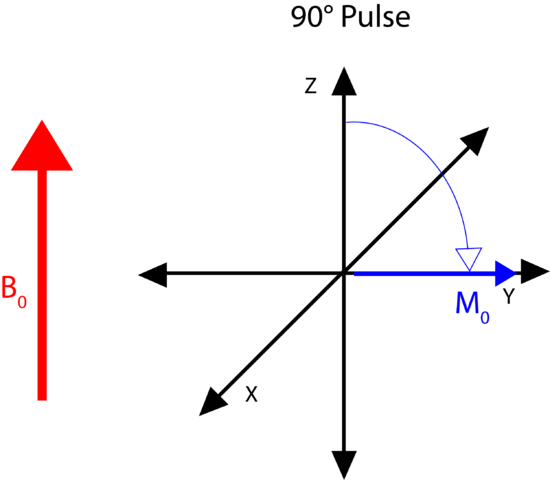
A pulse is a collection of oscillating waves with a broad range of frequencies (~1/4*pulse length) used to rotated the bulk magnetization. Pulses are described using two parameters, the angle and the phase. Typically, the angle and the phase are shown above the pulse. The angle can vary from 0°-180° While the phase can take on values from 0°-360°. Commonly the phase of the pulse is referred to the axis along which the \(B_1\) field is applied. For instance, shown below are the effects of a 90 pulse with a phase along x axis. This rotates the magnetization down along the y axis (right hand rule). While this example is fairly straightforward, pulse phases can become incredibly complex. More information about pulse phases will be covered in the phase cycling section. Pulses may be refereed to by just their angle ("a nintey pulse"), their angle in radians (a \(\frac{\pi}{2}\) "pi over two pulse") or their angle and phase "ninety x", (90°)x.

Acquisition
Now we move further to the right, increasing in time and see a squiggly line. This line represents the signal, which shows decay, as expected from T2 and T2* relaxation.
Multiple Pulse Sequences
Most pulse sequences have more than one pulse, which add a degree of complexity in to interpretations of the pulse sequence. Using multiple pulses have many advantageous including separation of NMR interactions, measuring relaxation timescales, and signal enhancement. Two additional features are present in multiple pulse experiments, delays and loops.

Delays
Delays are times when pulsing and detection are not occurring and are very important in pulse sequences, as separation of NMR interactions require precise timings. Additionally, creating proper delays can preserve select information as well as enhance signals. Delays are often referred to as "times". Below is a list of common delays:
- Relaxation Delay: Amount of time needed to wait before the next experiment can begin. Typically this is on the order 3-5 T1.
- Rotor Synchronized Delay (pulses): These delays are set so pulses remain centered in time with an integer multiple of the rotor period. Delays will then be:
\[Delay=n*\tau_r-\frac{1}{2}(P_i+P_f)\]
where \(n\) is an integer number, \(\tau_r\) is the spinning speed, Pi is the pulse length of the pulse before the delay and Pf is the pulse length of the pulse after the delay.
- Evolution (time) Delay: This is time during which the magnetization is precessing to satisfy the an equation relating to the separation of a variable.
- Storage (time) Delay: This is the time at which the bulk magnetization is stored along the external magnetic field to allow for sample manipulation, such a hopping or flipping.
Loops
Loops are repeating parts of the pulse sequence. They are typically employed in sequences to boost the S/N.
Echoes
Echoes are appear in pulse sequences as 2 FIDs placed in opposite directions. Figure 3 shows what an echo looks like during the CPMG loop.

