NMR Spectroscopy in Lab: Complications

There will be cases in which you already know what the structure might be. In these cases:

• One of the most complicated problems to deal with is the analysis of a mixture. This situation is not uncommon when students run reactions in lab and analyse the data.
  • Remember that integration ratios are really only meaningful within a single compound. If your NMR sample contains some benzene (C₆H₆) and some acetone (CH₃COCH₃), and there is a peak at 7.15 that integrates to 1 proton and a peak at 2.10 ppm integrating to 6 protons, it might mean there are 6 protons in acetone and 1 in benzene, but you can tell that isn't true by looking at the structure. There must be six times as many acetone molecules as benzene molecules in the sample.

    There are six protons in the benzene, and they should all show up near 7 ppm. There are six protons in acetone, and they should all show up near 2 ppm. Assuming that small integral of 1H for the benzene is really supposed to be 6H, then the large integral of 6H for the acetone must also represent six times as many hydrogens, too. It would be 36 H. There are only six hydrogens in acetone, so it must represent six times as many acetone molecules as there are benzenes.

    However, comparing the ratio of two integrals for two different compounds can give you the ratio of the two compounds in solution, just as we could determine the ratio of benzene to acetone in the mixture described above.

    We will look at two examples of sample mixtures that could arise in lab. Results like these are pretty common events in the labIn the first example, a student tried to carry out the following reaction, a borohydride reduction of an aldehyde. The borohydride should give a hydride anion to the C=O carbon; washing with water should then supply a proton to the oxygen, giving an alcohol.

    

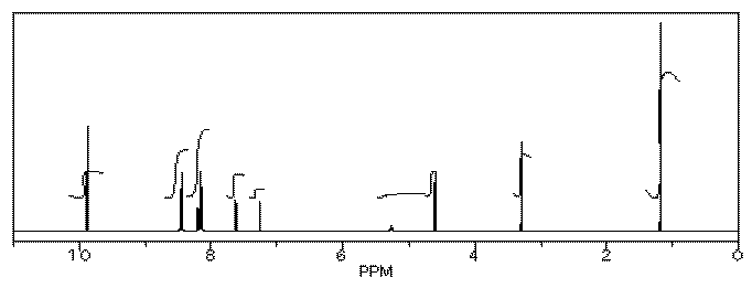
    Her reaction produced the following spectrum.

    

    (simulated data)

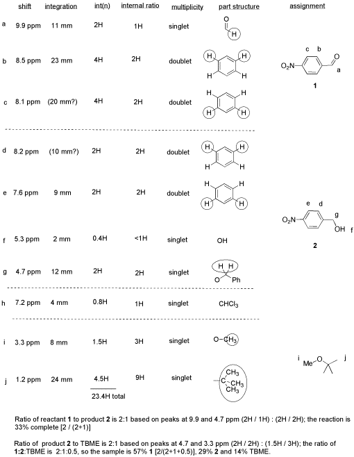
    From this data, she produced the table below.

    

    Notice how she calculated that ratio. She found a peak in molecule 1, the aldehyde, that she was pretty sure corresponded to the aldehydic hydrogen, the H attached to the C=O; in other words, the CH=O. She found another peak from molecule 2, the alcohol, that she was pretty sure represented the two hydrogens on the carbon attached to oxygen, the CH₂-O.

    The integrals for those two peaks are equal. They are both 2H in her table. However, she notes that within each molecule, the first integral really represents 1H and the second represents 2H. That means there must be twice as many of molecule 1 as there are molecule 2. That way, there would be 2 x CH=O, and its integral would be the same as the 1 x CH₂-O in the other molecule.

    One way to approach this kind of problem is to:

    • So there is twice as much aldehyde as alcohol in the mixture. In terms of these two compounds alone, she has 33% alcohol and 66% aldehyde. That's ( 1/(1+2) ) x100% for the alcohol, and ( 2/(1+2) ) x100% for the aldehyde. That calculation just represents the amount of individual component divided by the total of the components she wants to compare.

      There are a number of things to take note of here.

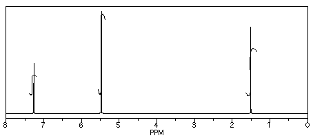
      • Another student carried out a similar reaction, shown below. He also finished the reaction by washing with water, but because methanol is soluble in water, he had to extract his product out of the water. He chose to use dichloromethane for that purpose.

        

        

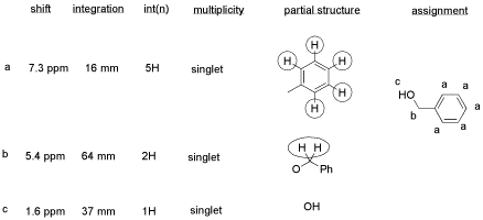
        From this data, he constructed the following table.

        

        There are some things to learn about this table, too.

        • This student might not get a very good grade; the sample does not even show up in the spectrum, so he lost it somewhere. But his analysis is also poor, so he will really get a terrible grade.

          Contributors and Attributions

          • Chris P Schaller, Ph.D., (College of Saint Benedict / Saint John's University)