1.59: The Quantum Bouncer Doesnʹt Bounce, Unless...
- Page ID
- 156289

\( \newcommand{\vecs}[1]{\overset { \scriptstyle \rightharpoonup} {\mathbf{#1}} } \)
\( \newcommand{\vecd}[1]{\overset{-\!-\!\rightharpoonup}{\vphantom{a}\smash {#1}}} \)
\( \newcommand{\id}{\mathrm{id}}\) \( \newcommand{\Span}{\mathrm{span}}\)
( \newcommand{\kernel}{\mathrm{null}\,}\) \( \newcommand{\range}{\mathrm{range}\,}\)
\( \newcommand{\RealPart}{\mathrm{Re}}\) \( \newcommand{\ImaginaryPart}{\mathrm{Im}}\)
\( \newcommand{\Argument}{\mathrm{Arg}}\) \( \newcommand{\norm}[1]{\| #1 \|}\)
\( \newcommand{\inner}[2]{\langle #1, #2 \rangle}\)
\( \newcommand{\Span}{\mathrm{span}}\)
\( \newcommand{\id}{\mathrm{id}}\)
\( \newcommand{\Span}{\mathrm{span}}\)
\( \newcommand{\kernel}{\mathrm{null}\,}\)
\( \newcommand{\range}{\mathrm{range}\,}\)
\( \newcommand{\RealPart}{\mathrm{Re}}\)
\( \newcommand{\ImaginaryPart}{\mathrm{Im}}\)
\( \newcommand{\Argument}{\mathrm{Arg}}\)
\( \newcommand{\norm}[1]{\| #1 \|}\)
\( \newcommand{\inner}[2]{\langle #1, #2 \rangle}\)
\( \newcommand{\Span}{\mathrm{span}}\) \( \newcommand{\AA}{\unicode[.8,0]{x212B}}\)
\( \newcommand{\vectorA}[1]{\vec{#1}} % arrow\)
\( \newcommand{\vectorAt}[1]{\vec{\text{#1}}} % arrow\)
\( \newcommand{\vectorB}[1]{\overset { \scriptstyle \rightharpoonup} {\mathbf{#1}} } \)
\( \newcommand{\vectorC}[1]{\textbf{#1}} \)
\( \newcommand{\vectorD}[1]{\overrightarrow{#1}} \)
\( \newcommand{\vectorDt}[1]{\overrightarrow{\text{#1}}} \)
\( \newcommand{\vectE}[1]{\overset{-\!-\!\rightharpoonup}{\vphantom{a}\smash{\mathbf {#1}}}} \)
\( \newcommand{\vecs}[1]{\overset { \scriptstyle \rightharpoonup} {\mathbf{#1}} } \)
\( \newcommand{\vecd}[1]{\overset{-\!-\!\rightharpoonup}{\vphantom{a}\smash {#1}}} \)
\(\newcommand{\avec}{\mathbf a}\) \(\newcommand{\bvec}{\mathbf b}\) \(\newcommand{\cvec}{\mathbf c}\) \(\newcommand{\dvec}{\mathbf d}\) \(\newcommand{\dtil}{\widetilde{\mathbf d}}\) \(\newcommand{\evec}{\mathbf e}\) \(\newcommand{\fvec}{\mathbf f}\) \(\newcommand{\nvec}{\mathbf n}\) \(\newcommand{\pvec}{\mathbf p}\) \(\newcommand{\qvec}{\mathbf q}\) \(\newcommand{\svec}{\mathbf s}\) \(\newcommand{\tvec}{\mathbf t}\) \(\newcommand{\uvec}{\mathbf u}\) \(\newcommand{\vvec}{\mathbf v}\) \(\newcommand{\wvec}{\mathbf w}\) \(\newcommand{\xvec}{\mathbf x}\) \(\newcommand{\yvec}{\mathbf y}\) \(\newcommand{\zvec}{\mathbf z}\) \(\newcommand{\rvec}{\mathbf r}\) \(\newcommand{\mvec}{\mathbf m}\) \(\newcommand{\zerovec}{\mathbf 0}\) \(\newcommand{\onevec}{\mathbf 1}\) \(\newcommand{\real}{\mathbb R}\) \(\newcommand{\twovec}[2]{\left[\begin{array}{r}#1 \\ #2 \end{array}\right]}\) \(\newcommand{\ctwovec}[2]{\left[\begin{array}{c}#1 \\ #2 \end{array}\right]}\) \(\newcommand{\threevec}[3]{\left[\begin{array}{r}#1 \\ #2 \\ #3 \end{array}\right]}\) \(\newcommand{\cthreevec}[3]{\left[\begin{array}{c}#1 \\ #2 \\ #3 \end{array}\right]}\) \(\newcommand{\fourvec}[4]{\left[\begin{array}{r}#1 \\ #2 \\ #3 \\ #4 \end{array}\right]}\) \(\newcommand{\cfourvec}[4]{\left[\begin{array}{c}#1 \\ #2 \\ #3 \\ #4 \end{array}\right]}\) \(\newcommand{\fivevec}[5]{\left[\begin{array}{r}#1 \\ #2 \\ #3 \\ #4 \\ #5 \\ \end{array}\right]}\) \(\newcommand{\cfivevec}[5]{\left[\begin{array}{c}#1 \\ #2 \\ #3 \\ #4 \\ #5 \\ \end{array}\right]}\) \(\newcommand{\mattwo}[4]{\left[\begin{array}{rr}#1 \amp #2 \\ #3 \amp #4 \\ \end{array}\right]}\) \(\newcommand{\laspan}[1]{\text{Span}\{#1\}}\) \(\newcommand{\bcal}{\cal B}\) \(\newcommand{\ccal}{\cal C}\) \(\newcommand{\scal}{\cal S}\) \(\newcommand{\wcal}{\cal W}\) \(\newcommand{\ecal}{\cal E}\) \(\newcommand{\coords}[2]{\left\{#1\right\}_{#2}}\) \(\newcommand{\gray}[1]{\color{gray}{#1}}\) \(\newcommand{\lgray}[1]{\color{lightgray}{#1}}\) \(\newcommand{\rank}{\operatorname{rank}}\) \(\newcommand{\row}{\text{Row}}\) \(\newcommand{\col}{\text{Col}}\) \(\renewcommand{\row}{\text{Row}}\) \(\newcommand{\nul}{\text{Nul}}\) \(\newcommand{\var}{\text{Var}}\) \(\newcommand{\corr}{\text{corr}}\) \(\newcommand{\len}[1]{\left|#1\right|}\) \(\newcommand{\bbar}{\overline{\bvec}}\) \(\newcommand{\bhat}{\widehat{\bvec}}\) \(\newcommand{\bperp}{\bvec^\perp}\) \(\newcommand{\xhat}{\widehat{\xvec}}\) \(\newcommand{\vhat}{\widehat{\vvec}}\) \(\newcommand{\uhat}{\widehat{\uvec}}\) \(\newcommand{\what}{\widehat{\wvec}}\) \(\newcommand{\Sighat}{\widehat{\Sigma}}\) \(\newcommand{\lt}{<}\) \(\newcommand{\gt}{>}\) \(\newcommand{\amp}{&}\) \(\definecolor{fillinmathshade}{gray}{0.9}\)The Earthʹs gravitational field is a confining potential and according to quantum mechanical principles, confinement gives rise to quantized energy levels. The one‐dimensional, time‐independent Schrödinger equation for a quantum object (quon, to use Nick Herbertʹs term) in the Earthʹs gravitational field near the surface is,
\[
\frac{-h^{2}}{8 \cdot \pi^{2} \cdot m} \cdot \frac{d^{2}}{d z^{2}} \Psi(z)+m \cdot g \cdot z \cdot \Psi(z)=E \cdot \Psi(z)
\nonumber \]
Here m is the mass of the quon, z its vertical distance from the Earthʹs surface, and g the acceleration due to gravity.
The solution to Schrödingerʹs equation for the mgz potential energy operator is well‐known. The energy eigenvalues and eigenfunctions are expressed in terms of the roots of the Airy function.
\[
\mathrm{E}_{\mathrm{i}}=\left(\frac{\mathrm{h}^{2} \cdot \mathrm{g}^{2} \cdot \mathrm{m}}{8 \cdot \pi^{2}}\right)^{\frac{1}{3}} \cdot \mathrm{a}_{\mathrm{i}} \qquad \Psi_{\mathrm{i}}(\mathrm{z})=\mathrm{N}_{\mathrm{i}} \cdot \mathrm{Ai}_{\mathrm{i}} \cdot\left[\left(\frac{8 \cdot \pi^{2} \cdot \mathrm{m}^{2} \cdot \mathrm{g}}{\mathrm{h}^{2}}\right)^{\frac{1}{3}} \cdot \mathrm{z}-\mathrm{a}_{\mathrm{i}}\right]
\nonumber \]
The first five roots of the Airy function are presented below.
\[
a_{1} :=2.33810 \quad a_{2} :=4.08794 \quad a_{3} :=5.52055 \quad a_{4} :=6.78670 \qquad a_{5} :=7.94413
\nonumber \]
Time dependence is introduced by multiplying the spatial wave function by \(\exp \left(-i \cdot \frac{2 \cdot \pi \cdot E_{i} \cdot t}{h}\right)\). The calculations that follow will be carried out in atomic units. In addition, the acceleration due to gravity and the quon mass will be set to unity for the sake of computational simplicity.
\[
\mathrm{h} :=2 \cdot \pi \quad \mathrm{g} :=1 \quad \mathrm{m} :=1 \quad \mathrm{i} :=1 \ldots 5 \\ \mathrm{E}_{\mathrm{i}} :=\left(\frac{\mathrm{h}^{2} \cdot \mathrm{g}^{2} \cdot \mathrm{m}}{8 \cdot \pi^{2}}\right)^{\frac{1}{3}} \cdot \mathrm{a}_{\mathrm{i}}
\nonumber \]
The wave functions for the ground state and first excited state are shown below.
\[
\Psi_{1}(z, t) :=1.6 \cdot \operatorname{Ai}\left[\left(\frac{8 \cdot \pi^{2} \cdot m^{2} \cdot g}{h^{2}}\right)^{\frac{1}{3}} \cdot z-a_{1}\right] \cdot e^{-i \cdot E_{1} \cdot t}
\nonumber \]
\[
\Psi_{2} (\mathrm{z}, \mathrm{t}) :=1.4 \cdot \mathrm{Ai}\left[\left(\frac{8 \cdot \pi^{2} \cdot \mathrm{m}^{2} \cdot \mathrm{g}}{\mathrm{h}^{2}}\right)^{\frac{1}{3}} \cdot \mathrm{z}-\mathrm{a}_{2}\right] \cdot \mathrm{e}^{-\mathrm{i} \cdot \mathrm{E}_{2} \cdot \mathrm{t}}
\nonumber \]
This excercise is usually called the quantum bouncer, but the first thing to stress is that these energy eigenfunctions are stationary states. In other words a quon in the Earthʹs gravitational field is in a state which is a weighted superposition of all possible positions above the surface of the earth which does not vary with time. It is not moving, it is not bouncing in any classical sense.
In other words the behavior of a quon is described by its time‐independent distribution function, \(|\Psi(z)|^{2}\), rather than by a trajectory ‐ a sequence of instantaneous positions and velocities. Quantum mechanics predicts the probability of finding the quon at any position above the Earthʹs surface, but the fact that it can be found at many different locations does not mean it is moving from one position to another. Quantum mechanics predicts the probability of observations, not what happens between two observations.
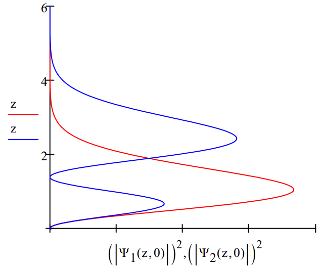
The position distribution functions, \(|\Psi(z)|^{2}\), for the ground‐ and first‐excited state are shown below.
The quantum bouncer doesnʹt ʺbounceʺ until it perturbed and forced into a superposition of eigenstates, for example, the ground‐ and first‐excited states
\[
\Phi(z, t) :=\frac{\Psi_{1}(z, t)+\Psi_{2}(z, t)}{\sqrt{2}}
\nonumber \]
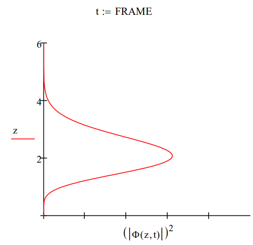
Below the quon distribution function is shown for three different times.
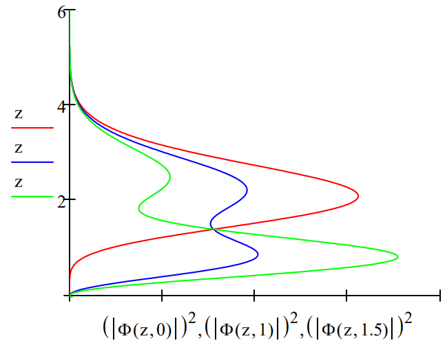
As the figure shows, now there is motion in the gravitational field. The quon is moving up and down, bouncing, because it is in a time‐dependent superposition of eigenstates.
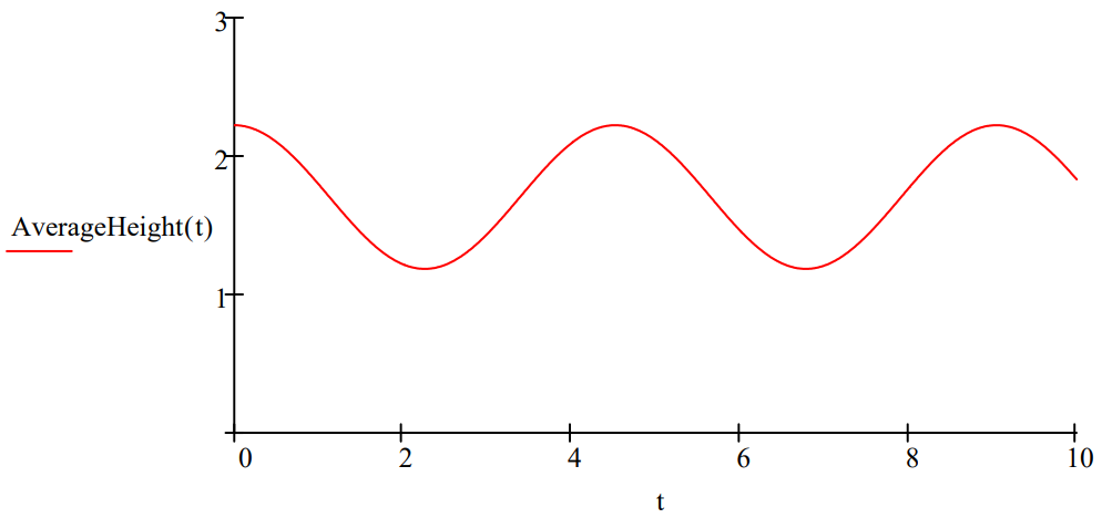
Another way this quantum mechanical ʺbouncing motionʺ can be illustrated is by displaying the time‐dependence of the average value of the position of the quon in the gravitational field.
\[
\text{AverageHeight}(\mathrm{t}) :=\int_{0}^{\infty} \mathrm{z} \cdot(|\Phi(z, t)|)^{2} \mathrm{d} \mathrm{z}
\nonumber \]
It is also possible to animate the time‐dependent superposition. Click on Tools, Animation, Record and follow the instructions in the dialog box. Choose From: 0, To: 100, At: 6 Frames/Sec.