1.38: Double‐Slit Experiment with Polarized Light

According to the Encyclopedia Britannica, Fresnel and Arago “using an apparatus based on Young’s [double‐slit] experiment” observed that “two beams polarized in mutually perpendicular planes never yield fringes.” The purpose of this tutorial is to examine this phenomenon from a quantum mechanical perspective.

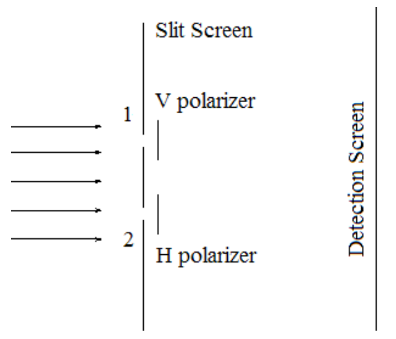
A schematic diagram of the double‐slit experiment with polarizers behind the slits is shown below. V and H stand for vertical and horizontal, respectively.

We begin with a review of the double‐slit experiment in the absence of the polarizers shown in the figure above. Illumination of the double‐slit screen with a coherent light source leads to a Schrödinger ʺcat stateʺ, in other words a superposition of the photon being localized at the both slits simultaneously. In effect, the slit screen performs a position measurement on the photons emanating from the light source.

\[
| \Psi \rangle=\frac{1}{\sqrt{2}}[ |x_{1}\rangle+| x_{2} \rangle ]
\nonumber \]

Here x₁ and x₂ are the positions of the two slits. For the sake of mathematical simplicity it is assumed that the slits are infinitesimally thin in the x‐direction and infinitely long in the y‐direction.

Because the slits localize the photon in the x‐direction the uncertainty principle demands a compensating delocalization in the x‐component of the momentum. To see this delocalization in momentum requires a momentum wave function, which is obtained by a Fourier transform of the position wave function given above. In this case the Fourier transform is simply the projection of the position wave function onto momentum space in atomic units (h = 2\(\pi\)).

\[
\Psi(p)=\langle p | \Psi\rangle=\frac{1}{\sqrt{2}}[\langle p | x_{1}\rangle+\langle p | x_{2}\rangle]=\frac{1}{2 \sqrt{\pi}}\left[\exp \left(-i p x_{1}\right)+\exp \left(-i p x_{2}\right)\right]
\nonumber \]

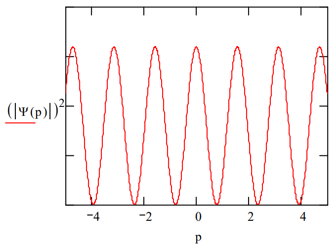
The diffraction pattern created by the double‐slit configuration of the screen is the square of the absolute magnitude of the momentum wave function, \(|\Psi(p)|^{2}\).

\[
|\langle p | \Psi\rangle|^{2}=\frac{1+\cos \left(p x_{1}\right) \cos \left(p x_{2}\right)+\sin \left(p x_{1}\right) \sin \left(p x_{2}\right)}{2 \pi}
\nonumber \]

The diffraction pattern below shows the required delocalization of momentum by the infinitesimally thin slits and interference fringes because the photon was localized at two spatial positions.

If slits of finite width were used the mathematics would be a little more complicated and lead to the following familiar diffraction pattern.

In the presence of the polarizing films, the spatial wave function becomes,

\[
| \Psi \rangle=\frac{1}{\sqrt{2}}[ |x_{1}\rangle | v \rangle+| x_{2} \rangle | h \rangle ]
\nonumber \]

where v and h represent the vertical and horizontal polarization states. Projecting this wave function onto momentum space yields,

\[
\Psi(p)=\langle p | \Psi\rangle=\frac{1}{\sqrt{2}}[\langle p | x_{1}\rangle | v\rangle+\langle p | x_{2}\rangle | h \rangle ]
\nonumber \]

The square of the absolute magnitude of the momentum wave function is, again, the diffraction pattern,

\[
|\langle p | \Psi\rangle|^{2}=\frac{1}{\sqrt{2}}\left[|\langle p | x_{1}\rangle|^{2}+|\langle p | x_{2}\rangle|^{2}\right]=\frac{1}{2 \pi}
\nonumber \]

We see that due to the presence of the polarizing films the interference terms (fringes) disappear.