1.39: The Consequences of Path Information in a Mach-Zehnder Interferometer
- Page ID
- 144053
\( \newcommand{\vecs}[1]{\overset { \scriptstyle \rightharpoonup} {\mathbf{#1}} } \)
\( \newcommand{\vecd}[1]{\overset{-\!-\!\rightharpoonup}{\vphantom{a}\smash {#1}}} \)
\( \newcommand{\id}{\mathrm{id}}\) \( \newcommand{\Span}{\mathrm{span}}\)
( \newcommand{\kernel}{\mathrm{null}\,}\) \( \newcommand{\range}{\mathrm{range}\,}\)
\( \newcommand{\RealPart}{\mathrm{Re}}\) \( \newcommand{\ImaginaryPart}{\mathrm{Im}}\)
\( \newcommand{\Argument}{\mathrm{Arg}}\) \( \newcommand{\norm}[1]{\| #1 \|}\)
\( \newcommand{\inner}[2]{\langle #1, #2 \rangle}\)
\( \newcommand{\Span}{\mathrm{span}}\)
\( \newcommand{\id}{\mathrm{id}}\)
\( \newcommand{\Span}{\mathrm{span}}\)
\( \newcommand{\kernel}{\mathrm{null}\,}\)
\( \newcommand{\range}{\mathrm{range}\,}\)
\( \newcommand{\RealPart}{\mathrm{Re}}\)
\( \newcommand{\ImaginaryPart}{\mathrm{Im}}\)
\( \newcommand{\Argument}{\mathrm{Arg}}\)
\( \newcommand{\norm}[1]{\| #1 \|}\)
\( \newcommand{\inner}[2]{\langle #1, #2 \rangle}\)
\( \newcommand{\Span}{\mathrm{span}}\) \( \newcommand{\AA}{\unicode[.8,0]{x212B}}\)
\( \newcommand{\vectorA}[1]{\vec{#1}} % arrow\)
\( \newcommand{\vectorAt}[1]{\vec{\text{#1}}} % arrow\)
\( \newcommand{\vectorB}[1]{\overset { \scriptstyle \rightharpoonup} {\mathbf{#1}} } \)
\( \newcommand{\vectorC}[1]{\textbf{#1}} \)
\( \newcommand{\vectorD}[1]{\overrightarrow{#1}} \)
\( \newcommand{\vectorDt}[1]{\overrightarrow{\text{#1}}} \)
\( \newcommand{\vectE}[1]{\overset{-\!-\!\rightharpoonup}{\vphantom{a}\smash{\mathbf {#1}}}} \)
\( \newcommand{\vecs}[1]{\overset { \scriptstyle \rightharpoonup} {\mathbf{#1}} } \)
\( \newcommand{\vecd}[1]{\overset{-\!-\!\rightharpoonup}{\vphantom{a}\smash {#1}}} \)
This tutorial deals with the effect of path information in a Mach-Zehnder interferometer (MZI). A related analysis involving the double-slit experiment is available in the preceding tutorial. We begin with an analysis of the operation of an equal arm MZI illuminated with diagonally polarized light.
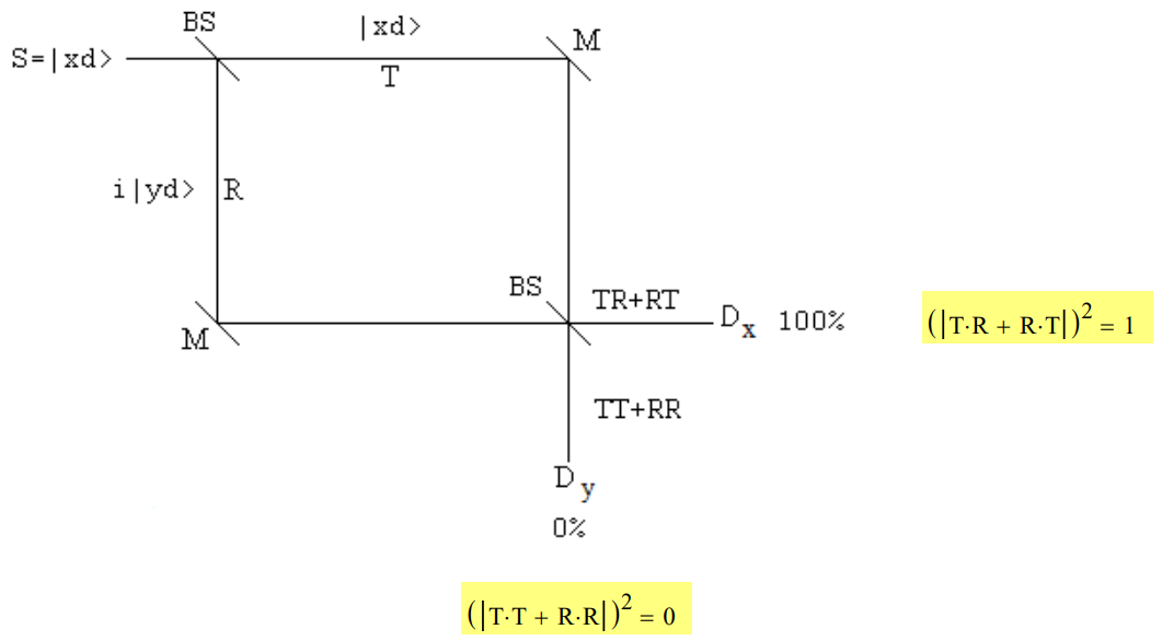
The source emits photons in the x-direction illuminating a 50/50 beam splitter (BS) which splits the beam into a superposition of propagation in the x- and y-directions. The reflected beam collects a 90 degree (\(\frac{\pi}{2}\), i) phase shift relative to the transmitted beam. Mirrors redirect the two beams to a second 50/50 BS. For an equal arm interferometer the photons are always registered at Dx and never at Dy. One way to explain this is shown in the figure below. A photon has two paths to each detector. At Dx the probability amplitudes of the photon's paths add in phase each being shifted by 90 degrees, resulting in constructive interference. At Dy the probability amplitudes are 180 degrees out of phase causing destructive interference. The beam splitters do not operate on the polarization states of the photons.
| Probability amplitude for photon transmission at a 50/50 beam splitter: \(T : = \frac{1}{\sqrt{2}}\) | Probability amplitude for photon reflection at a 50/50 beam splitter: \(R : = \frac{i}{\sqrt{2}}\) |

An equivalent matrix mechanics analysis uses vectors to represent the photon's direction of propagation and polarization, and matrices to represent the objects that operate on the photon states, such as beam splitters and mirrors. In the analyses which follow a photon can be moving in the x- or y-direction with diagonal, horizontal or vertical polarization.
Propagation states:
\[
\mathrm{x} :=\left( \begin{array}{l}{1} \\ {0}\end{array}\right) \qquad \mathrm{y} :=\left( \begin{array}{l}{0} \\ {1}\end{array}\right)
\nonumber \]
Polarization states:
\[
\mathrm{d} :=\frac{1}{\sqrt{2}} \cdot \left( \begin{array}{l}{1} \\ {1}\end{array}\right) \qquad \mathrm{h} :=\left( \begin{array}{l}{1} \\ {0}\end{array}\right) \qquad \mathrm{v} :=\left( \begin{array}{l}{0} \\ {1}\end{array}\right)
\nonumber \]
The Appendix shows how the propagation and polarization states are written as a composite state using tensor multiplication of vectors.
\[
\mathrm{xd} :=\frac{1}{\sqrt{2}} \cdot \left( \begin{array}{l}{1} \\ {1} \\ {0} \\ {0}\end{array}\right) \qquad \mathrm{yd} :=\frac{1}{\sqrt{2}} \cdot \left( \begin{array}{l}{0} \\ {0} \\ {1} \\ {1}\end{array}\right)
\nonumber \]
\[
\mathrm{xh} :=\left( \begin{array}{l}{1} \\ {0} \\ {0} \\ {0}\end{array}\right) \qquad \mathrm{yh} :=\left( \begin{array}{c}{0} \\ {0} \\ {1} \\ {0}\end{array}\right)
\nonumber \]
\[
\mathrm{xv} :=\left( \begin{array}{l}{0} \\ {1} \\ {0} \\ {0}\end{array}\right) \qquad \mathrm{yv} :=\left( \begin{array}{l}{0} \\ {0} \\ {0} \\ {1}\end{array}\right)
\nonumber \]
The beam splitters and mirrors operate on the photon's direction of propagation but not on its polarization. The identity (do nothing) operates on the second degree of freedom, polarization.
Beam splitter:
\[
\frac{1}{\sqrt{2}} \cdot \left( \begin{array}{ll}{1} & {\mathrm{i}} \\ {\mathrm{i}} & {1}\end{array}\right)
\nonumber \]
Mirror:
\[
\left( \begin{array}{ll}{0} & {1} \\ {1} & {0}\end{array}\right)
\nonumber \]
Identity:
\[
\left( \begin{array}{ll}{1} & {0} \\ {0} & {1}\end{array}\right)
\nonumber \]
Kronecker, Mathcad's command for tensor multiplication of matrices, insures that the beam splitters and mirrors operate on direction of motion, and that photon polarization evolves unchanged. See the Appendix for the details of the tensor product of two matrices.
\[
\mathrm{BS} :=\text { kronecker }\left[\frac{1}{\sqrt{2}} \cdot \left( \begin{array}{ll}{1} & {\mathrm{i}} \\ {\mathrm{i}} & {1}\end{array}\right), \left( \begin{array}{ll}{1} & {0} \\ {0} & {1}\end{array}\right)\right]
\nonumber \]
\[
\text{M} :=\text { kronecker } \left[\left( \begin{array}{cc}{0} & {1} \\ {1} & {0}\end{array}\right), \left( \begin{array}{ll}{1} & {0} \\ {0} & {1}\end{array}\right) \right]
\nonumber \]
The probability that the photon will be moving in the x-direction after the second BS and detected at Dx is 1. The probability it will be registered at Dy is 0.
\[
\left(|\mathrm{xd}^{\mathrm{T}} \cdot \mathrm{BS} \cdot \mathrm{M} \cdot \mathrm{BS} \cdot \mathrm{xd}|\right)^{2}=1
\nonumber \]
\[
\left(|\mathrm{yd}^{\mathrm{T}} \cdot \mathrm{BS} \cdot \mathrm{M} \cdot \mathrm{BS} \cdot \mathrm{xd}|\right)^{2}=0
\nonumber \]
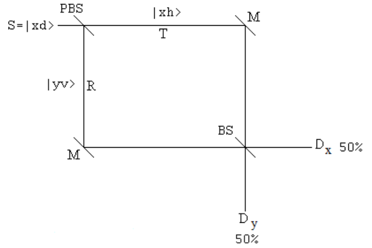
Photon path information can be added by replacing the first BS with a polarizing beam splitter (PBS), which transmits horizontal polarization and reflects vertical polarization. There is no phase shift between transmission and reflection in a PBS.

The matrix representing a PBS can be constructed by considering the fate of the individual photon states encountering a PBS. The individual terms are from right to left. For example, |yv> <yx| means xv --> yv.
\[
\widehat{P B S}=| x h \rangle\langle x h|+| y v\rangle\langle x v|+| y h\rangle\langle y h|+| x v\rangle\langle y v |
\nonumber \]
\[
\mathrm{PBS} :=\mathrm{xh} \cdot \mathrm{xh}^{\mathrm{T}}+\mathrm{yv} \cdot \mathrm{xv}^{\mathrm{T}}+\mathrm{yh} \cdot \mathrm{yh}^{\mathrm{T}}+\mathrm{xv} \cdot \mathrm{yv}^{\mathrm{T}}=\left( \begin{array}{cccc}{1} & {0} & {0} & {0} \\ {0} & {0} & {0} & {1} \\ {0} & {0} & {1} & {0} \\ {0} & {1} & {0} & {0}\end{array}\right)
\nonumber \]
After the PBS the diagonally polarized photon is in a superposition of being transmitted with horizontal polarization and reflected with vertical polarization. In other words the two photon paths have been labeled with orthogonal polarization states; path information is available.
\[
\operatorname{PBS} \cdot \mathrm{x} \mathrm{d}=\left( \begin{array}{c}{0.707} \\ {0} \\ {0} \\ {0.707}\end{array}\right)
\nonumber \]
\[
\frac{1}{\sqrt{2}} \cdot(\mathrm{xh}+\mathrm{yv})=\left( \begin{array}{c}{0.707} \\ {0} \\ {0} \\ {0.707}\end{array}\right)
\nonumber \]
The following calculations show that this path information destroys the interference observed in the original MZI. Now both detectors fire with equal probability as shown in the diagram above. Half the time the photon is detected at Dx with either horizontal or vertical polarization, and half the time the photon is detected at Dy with horizontal or vertical polarization. This occurs because the path tags are orthogonal polarization states.
\[
\left(|\mathrm{xv}^{\mathrm{T}} \cdot \mathrm{BS} \cdot \mathrm{M} \cdot \mathrm{PBS} \cdot \mathrm{xd}|\right)^{2}=0.25 \qquad \left(|\mathrm{xh}^{\mathrm{T}} \cdot \mathrm{BS} \cdot \mathrm{M} \cdot \mathrm{PBS} \cdot \mathrm{xd}|\right)^{2}=0.25
\nonumber \]
\[
\left(|\mathrm{yv}^{\mathrm{T}} \cdot \mathrm{BS} \cdot \mathrm{M} \cdot \mathrm{PBS} \cdot \mathrm{xd}|\right)^{2}=0.25 \qquad \left(|\mathrm{yh}^{\mathrm{T}} \cdot \mathrm{BS} \cdot \mathrm{M} \cdot \mathrm{PBS} \cdot \mathrm{xd}|\right)^{2}=0.25
\nonumber \]
An algebraic representation of the steps from source to detectors gives the same numbers when the magnitudes of the probability amplitudes are squared to give the probabilities for each possible measurement outcome at Dx and Dy.
\[
| x d \rangle \stackrel{P B S}{\longrightarrow} \frac{1}{\sqrt{2}}[ | x h\rangle+| y v \rangle ] \xrightarrow[B S]{M} \frac{1}{\sqrt{2}}[i | x h\rangle+| y h \rangle ]
\nonumber \]
If the PBS is illuminated with horizontally or vertically polarized photons, there is only one path to the beam splitter in front of the detectors. Again both detectors fire with equal probability because there is no opportunity for path interference.
Horizontally polarized source:
\[
\left(|\mathrm{xh}^{\mathrm{T}} \cdot \mathrm{BS} \cdot \mathrm{M} \cdot \mathrm{PBS} \cdot \mathrm{xh}|\right)^{2}=0.5 \qquad \left[ | \operatorname{yh}^{\mathrm{T}} \cdot(\mathrm{BS} \cdot \mathrm{M} \cdot \mathrm{PBS}) \cdot \mathrm{xh}\right] ]^{2}=0.5
\nonumber \]
\[
| x h \rangle \stackrel{P B S}{\longrightarrow} | x h\rangle \xrightarrow[B S]{M} \frac{1}{\sqrt{2}}[i | x h\rangle+| y h \rangle ]
\nonumber \]
Vertically polarized source:
\[
\left(|\mathrm{xv}^{\mathrm{T}} \cdot \mathrm{BS} \cdot \mathrm{M} \cdot \mathrm{PBS} \cdot \mathrm{xv}|\right)^{2}=0.5 \qquad \left[ | \operatorname{yv}^{\mathrm{T}} \cdot(\mathrm{BS} \cdot \mathrm{M} \cdot \mathrm{PBS}) \cdot \mathrm{xv}\right] ]^{2}=0.5
\nonumber \]
\[
| x v \rangle \stackrel{P B S}{\longrightarrow} | y v \rangle \xrightarrow[B S]{M} \frac{1}{\sqrt{2}}[i | x v\rangle+i| y h \rangle ]
\nonumber \]
Appendix
Tensor products for the various propagation/polarization states are formed as follows:
\[
| x d \rangle=\left( \begin{array}{l}{1} \\ {0}\end{array}\right) \otimes \frac{1}{\sqrt{2}} \left( \begin{array}{l}{1} \\ {1}\end{array}\right)=\frac{1}{\sqrt{2}} \left( \begin{array}{l}{1} \\ {1} \\ {0} \\ {0}\end{array}\right) \qquad | y d \rangle=\left( \begin{array}{l}{0} \\ {1}\end{array}\right) \otimes \frac{1}{\sqrt{2}} \left( \begin{array}{l}{1} \\ {1}\end{array}\right)=\frac{1}{\sqrt{2}} \left( \begin{array}{l}{0} \\ {0} \\ {1} \\ {1}\end{array}\right)
\nonumber \]
\[
| x h \rangle=\left( \begin{array}{l}{1} \\ {0}\end{array}\right) \otimes \left( \begin{array}{l}{1} \\ {0}\end{array}\right)=\left( \begin{array}{l}{1} \\ {0} \\ {0} \\ {0}\end{array}\right) \qquad | x v \rangle=\left( \begin{array}{l}{1} \\ {0}\end{array}\right) \otimes \left( \begin{array}{l}{0} \\ {1}\end{array}\right)=\left( \begin{array}{l}{0} \\ {1} \\ {0} \\ {0}\end{array}\right)
\nonumber \]
\[
| y h \rangle=\left( \begin{array}{l}{0} \\ {1}\end{array}\right) \otimes \left( \begin{array}{l}{1} \\ {0}\end{array}\right)=\left( \begin{array}{l}{0} \\ {0} \\ {1} \\ {0}\end{array}\right) \qquad | y v \rangle=\left( \begin{array}{l}{0} \\ {1}\end{array}\right) \otimes \left( \begin{array}{l}{0} \\ {1}\end{array}\right)=\left( \begin{array}{l}{0} \\ {0} \\ {0} \\ {1}\end{array}\right)
\nonumber \]
An example of the tensor product of two matrices:
\[
\left( \begin{array}{ll}{a} & {b} \\ {c} & {d}\end{array}\right) \otimes \left( \begin{array}{ll}{w} & {x} \\ {y} & {z}\end{array}\right) =\left( \begin{array}{ll}{a \left( \begin{array}{cc}{w} & {x} \\ {y} & {z}\end{array}\right)} & {b \left( \begin{array}{cc}{w} & {x} \\ {y} & {z}\end{array}\right)} \\ {c \left( \begin{array}{ll}{w} & {x} \\ {y} & {z}\end{array}\right)} & {d \left( \begin{array}{cc}{w} & {x} \\ {y} & {z}\end{array}\right)}\end{array}\right)=\left( \begin{array}{llll}{a w} & {a x} & {b w} & {b x} \\ {a y} & {a z} & {b y} & {b z} \\ {c w} & {c x} & {d w} & {d x} \\ {c y} & {c z} & {d y} & {d z}\end{array}\right)
\nonumber \]

