1.37: The Double-Slit Experiment
- Page ID
- 144005
\( \newcommand{\vecs}[1]{\overset { \scriptstyle \rightharpoonup} {\mathbf{#1}} } \)
\( \newcommand{\vecd}[1]{\overset{-\!-\!\rightharpoonup}{\vphantom{a}\smash {#1}}} \)
\( \newcommand{\id}{\mathrm{id}}\) \( \newcommand{\Span}{\mathrm{span}}\)
( \newcommand{\kernel}{\mathrm{null}\,}\) \( \newcommand{\range}{\mathrm{range}\,}\)
\( \newcommand{\RealPart}{\mathrm{Re}}\) \( \newcommand{\ImaginaryPart}{\mathrm{Im}}\)
\( \newcommand{\Argument}{\mathrm{Arg}}\) \( \newcommand{\norm}[1]{\| #1 \|}\)
\( \newcommand{\inner}[2]{\langle #1, #2 \rangle}\)
\( \newcommand{\Span}{\mathrm{span}}\)
\( \newcommand{\id}{\mathrm{id}}\)
\( \newcommand{\Span}{\mathrm{span}}\)
\( \newcommand{\kernel}{\mathrm{null}\,}\)
\( \newcommand{\range}{\mathrm{range}\,}\)
\( \newcommand{\RealPart}{\mathrm{Re}}\)
\( \newcommand{\ImaginaryPart}{\mathrm{Im}}\)
\( \newcommand{\Argument}{\mathrm{Arg}}\)
\( \newcommand{\norm}[1]{\| #1 \|}\)
\( \newcommand{\inner}[2]{\langle #1, #2 \rangle}\)
\( \newcommand{\Span}{\mathrm{span}}\) \( \newcommand{\AA}{\unicode[.8,0]{x212B}}\)
\( \newcommand{\vectorA}[1]{\vec{#1}} % arrow\)
\( \newcommand{\vectorAt}[1]{\vec{\text{#1}}} % arrow\)
\( \newcommand{\vectorB}[1]{\overset { \scriptstyle \rightharpoonup} {\mathbf{#1}} } \)
\( \newcommand{\vectorC}[1]{\textbf{#1}} \)
\( \newcommand{\vectorD}[1]{\overrightarrow{#1}} \)
\( \newcommand{\vectorDt}[1]{\overrightarrow{\text{#1}}} \)
\( \newcommand{\vectE}[1]{\overset{-\!-\!\rightharpoonup}{\vphantom{a}\smash{\mathbf {#1}}}} \)
\( \newcommand{\vecs}[1]{\overset { \scriptstyle \rightharpoonup} {\mathbf{#1}} } \)
\( \newcommand{\vecd}[1]{\overset{-\!-\!\rightharpoonup}{\vphantom{a}\smash {#1}}} \)
\(\newcommand{\avec}{\mathbf a}\) \(\newcommand{\bvec}{\mathbf b}\) \(\newcommand{\cvec}{\mathbf c}\) \(\newcommand{\dvec}{\mathbf d}\) \(\newcommand{\dtil}{\widetilde{\mathbf d}}\) \(\newcommand{\evec}{\mathbf e}\) \(\newcommand{\fvec}{\mathbf f}\) \(\newcommand{\nvec}{\mathbf n}\) \(\newcommand{\pvec}{\mathbf p}\) \(\newcommand{\qvec}{\mathbf q}\) \(\newcommand{\svec}{\mathbf s}\) \(\newcommand{\tvec}{\mathbf t}\) \(\newcommand{\uvec}{\mathbf u}\) \(\newcommand{\vvec}{\mathbf v}\) \(\newcommand{\wvec}{\mathbf w}\) \(\newcommand{\xvec}{\mathbf x}\) \(\newcommand{\yvec}{\mathbf y}\) \(\newcommand{\zvec}{\mathbf z}\) \(\newcommand{\rvec}{\mathbf r}\) \(\newcommand{\mvec}{\mathbf m}\) \(\newcommand{\zerovec}{\mathbf 0}\) \(\newcommand{\onevec}{\mathbf 1}\) \(\newcommand{\real}{\mathbb R}\) \(\newcommand{\twovec}[2]{\left[\begin{array}{r}#1 \\ #2 \end{array}\right]}\) \(\newcommand{\ctwovec}[2]{\left[\begin{array}{c}#1 \\ #2 \end{array}\right]}\) \(\newcommand{\threevec}[3]{\left[\begin{array}{r}#1 \\ #2 \\ #3 \end{array}\right]}\) \(\newcommand{\cthreevec}[3]{\left[\begin{array}{c}#1 \\ #2 \\ #3 \end{array}\right]}\) \(\newcommand{\fourvec}[4]{\left[\begin{array}{r}#1 \\ #2 \\ #3 \\ #4 \end{array}\right]}\) \(\newcommand{\cfourvec}[4]{\left[\begin{array}{c}#1 \\ #2 \\ #3 \\ #4 \end{array}\right]}\) \(\newcommand{\fivevec}[5]{\left[\begin{array}{r}#1 \\ #2 \\ #3 \\ #4 \\ #5 \\ \end{array}\right]}\) \(\newcommand{\cfivevec}[5]{\left[\begin{array}{c}#1 \\ #2 \\ #3 \\ #4 \\ #5 \\ \end{array}\right]}\) \(\newcommand{\mattwo}[4]{\left[\begin{array}{rr}#1 \amp #2 \\ #3 \amp #4 \\ \end{array}\right]}\) \(\newcommand{\laspan}[1]{\text{Span}\{#1\}}\) \(\newcommand{\bcal}{\cal B}\) \(\newcommand{\ccal}{\cal C}\) \(\newcommand{\scal}{\cal S}\) \(\newcommand{\wcal}{\cal W}\) \(\newcommand{\ecal}{\cal E}\) \(\newcommand{\coords}[2]{\left\{#1\right\}_{#2}}\) \(\newcommand{\gray}[1]{\color{gray}{#1}}\) \(\newcommand{\lgray}[1]{\color{lightgray}{#1}}\) \(\newcommand{\rank}{\operatorname{rank}}\) \(\newcommand{\row}{\text{Row}}\) \(\newcommand{\col}{\text{Col}}\) \(\renewcommand{\row}{\text{Row}}\) \(\newcommand{\nul}{\text{Nul}}\) \(\newcommand{\var}{\text{Var}}\) \(\newcommand{\corr}{\text{corr}}\) \(\newcommand{\len}[1]{\left|#1\right|}\) \(\newcommand{\bbar}{\overline{\bvec}}\) \(\newcommand{\bhat}{\widehat{\bvec}}\) \(\newcommand{\bperp}{\bvec^\perp}\) \(\newcommand{\xhat}{\widehat{\xvec}}\) \(\newcommand{\vhat}{\widehat{\vvec}}\) \(\newcommand{\uhat}{\widehat{\uvec}}\) \(\newcommand{\what}{\widehat{\wvec}}\) \(\newcommand{\Sighat}{\widehat{\Sigma}}\) \(\newcommand{\lt}{<}\) \(\newcommand{\gt}{>}\) \(\newcommand{\amp}{&}\) \(\definecolor{fillinmathshade}{gray}{0.9}\)Thomas Young used the double-slit experiment to establish the wave nature of light. Richard Feynman used it to demonstrate the superposition principle as the paradigm of all quantum mechanical phenomena, illustrating wave-particle duality as stated above: between release and detection quons behave as waves.
The Experiment
The slit screen on the left produces the diffraction pattern on the right when illuminated with a coherent radiation source.

The Quantum Mechanical Explanation
Illumination of a double-slit screen with a coherent light source leads to a Schrödinger "cat state", in other words a superposition of the photon being localized at both slits simultaneously.
\[| \Psi \rangle=\frac{1}{\sqrt{2}}[ |x_{1}\rangle+| x_{2} \rangle ] \nonumber \]
Here x1 and x2 are positions of the two slits. It is assumed initially, for the sake of mathematical simplicity, that the slits are infinitesimally thin in the x-direction and infinitely long in the y-direction.
Because the slits localize the photon in the x-direction the uncertainty principle \(\left(\Delta \mathrm{x} \Delta \mathrm{p}_{\mathrm{x}}>\frac{\mathrm{h}}{4 \pi}\right)\) demands a compensating delocalization in the x-component of the momentum. To see this delocalization in momentum requires a momentum wave function, which is obtained by a Fourier transform of the position wave function given above.
In this case the Fourier transform is simply the projection of the position wave function onto momentum space. See the Appendix for further information on the Fourier transform.
\[\langle p | \Psi\rangle=\frac{1}{\sqrt{2}}[\langle p | x_{1}\rangle+\langle p | x_{2}\rangle]=\frac{1}{2 \sqrt{\pi}}\left[\exp \left(-\frac{i p x_{1}}{\hbar}\right)+\exp \left(-\frac{i p x_{2}}{\hbar}\right)\right] \nonumber \]
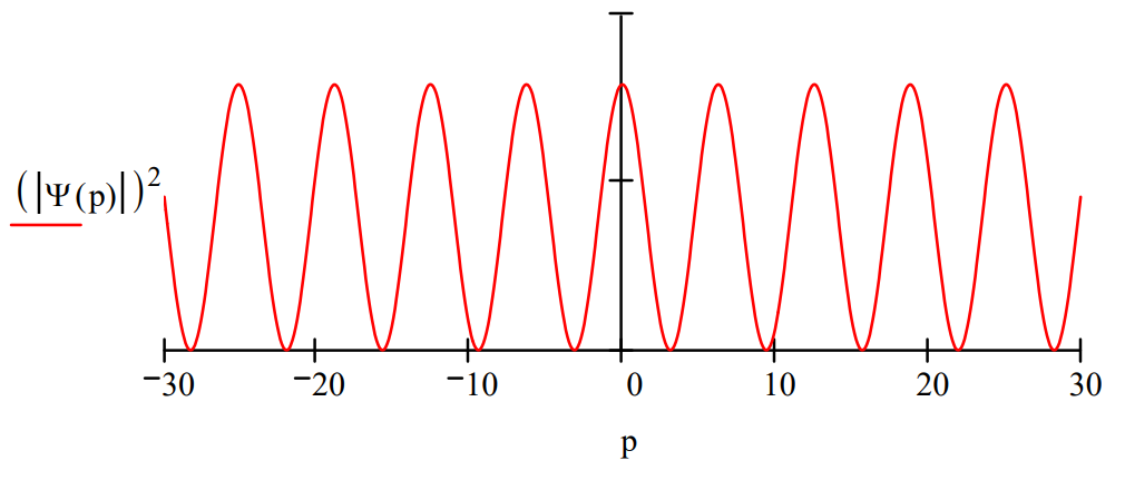
The quantum mechanical interpretation of the double-slit experiment, or any diffraction experiment for that matter, is that the diffraction pattern is actually the momentum distribution function, \(|<p| \Psi>\left.\right|^{2}\). This is illustrated below. The following calculations are carried out in atomic units (h = 2 \(\pi\)).
| Position of first slit: \(x_{1} : = 0\) | Position of second slit: \(x_{2} : = 1\) |
\[\mathrm{p} :=-30,-29.9 \ldots30 \quad \Psi(\mathrm{p}) :=\frac{\frac{1}{\sqrt{2 \cdot \pi}} \cdot \exp \left(-\mathrm{i} \cdot \mathrm{p} \cdot \mathrm{x}_{1}\right)+\frac{1}{\sqrt{2 \cdot \pi}} \cdot \exp \left(-\mathrm{i} \cdot \mathrm{p} \cdot \mathrm{x}_{2}\right)}{\sqrt{2}} \nonumber \]

The momentum distribution shows interference fringes because the photons were localized in space at two positions: the maxima represent constructive interference and the minima destructive interference. Notice also that the momentum distribution in the x-direction is completely delocalized; it shows no sign of attenuating at large momentum values. This is due to the fact that under the present model the photons are precisely localized at x1 and x2 - in other words the slits are infinitesimally thin in the x-direction as specified above.
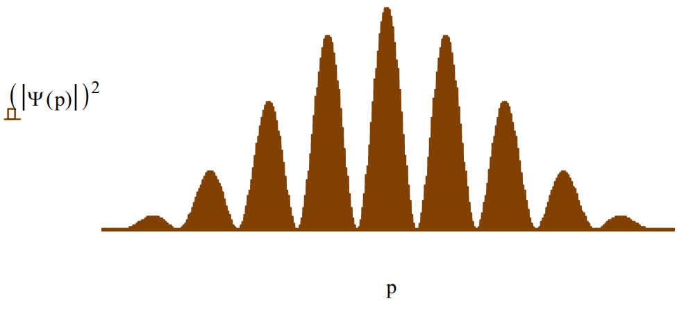
This of course is not an adequate representation of the actual double-slit diffraction pattern because any real slit has a finite size in both directions. It's really not a problem that the slit is infinite in the y-direction, because that means the photon is simply not localized in that direction. So all we need to do to get a more realistic double-slit diffraction pattern is make the slits finite (not infinitesimal) in the x-direction. This is accomplished by giving the slits a finite width, \(\delta\), in the x-direction, and recalculating the momentum wave function.
Slit width:
\[\delta :=0.2 \quad \Psi(\mathrm{p}) := \frac{\int_{\mathrm{x}_{1}-\frac{\delta}{2}}^{\mathrm{x}_{1}+\frac{\delta}{2}} \frac{1}{\sqrt{2 \cdot \pi}} \cdot \exp (-\mathrm{i} \cdot \mathrm{p} \cdot \mathrm{x}) \cdot \frac{1}{\sqrt{\delta}} \mathrm{d} \mathrm{x}+\int_{\mathrm{x}_{2}-\frac{\delta}{2}}^{\mathrm{x}_{2}+\frac{\delta}{2}} \frac{1}{\sqrt{2 \cdot \pi}} \cdot \exp (-\mathrm{i} \cdot \mathrm{p} \cdot \mathrm{x}) \cdot \frac{1}{\sqrt{\delta}} \mathrm{d} \mathrm{x}}{\sqrt{2}} \nonumber \]

In summary, the quantum mechanical interpretation of the double-slit experiment is that position is measured at the slit screen and momentum is measured at the detection screen. Position and momentum are conjugate observables which are connected by a Fourier transform and governed by the uncertainty principle. Knowing the slit screen geometry makes it possible to calculate the momentum distribution at the detection screen. Varying the slit width, \(\delta\), gives a clear and simple demonstration of the uncertainty principle in action. Narrow slit widths give broad momentum distributions and wide slit widths give narrow momentum distributions.

