1.101: Related Analysis of the Stern-Gerlach Experiment

Silver atoms are deflected by an inhomogeneous magnetic field because of the two-valued magnetic moment associated with their unpaired 5s electron ([Kr]5s¹4d¹⁰). The beam of silver atoms entering the Stern-Gerlach magnet oriented in the z-direction (SGZ) on the left is unpolarized. This means it is a mixture of randomly polarized Ag atoms. A mixture cannot be represented by a wave function, it requires a density matrix, as will be shown later.

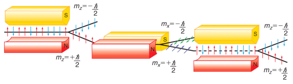
This situation is exactly analogous to the three-polarizer demonstration. Light emerging from an incadescent light bulb is unpolarized, a mixture of all possible polarization angles, so we can't write a wave function for it. The first Stern-Gerlach magnet plays the same role as the first polarizer, it forces the Ag atoms into one of measurement eigenstates - spin-up or spin-down in the z-direction. The only difference is that in the three-polarizer demonstration only one state was created - vertical polarization. Both demonstrations illustrate that the only values that are observed in an experiment are the eigenvalues of the measurement operator.

To continue with the analysis of the Stern-Gerlach demonstration we need vectors to represent the various spin states of the Ag atoms.

Spin Eigenfunctions

Spin-up in the z-direction:	\(\alpha_{\mathrm{Z}} :=\left(\begin{array}{l}{1} \\ {0}\end{array}\right)\)
Spin-down in the z-direction:	\(\beta_{\mathrm{z}} :=\left(\begin{array}{l}{0} \\ {1}\end{array}\right)\)
Spin-up in the x-direction:	\(\alpha_{\mathrm{x}} :=\frac{1}{\sqrt{2}} \cdot\left(\begin{array}{l}{1} \\ {1}\end{array}\right)\)
Spin-down in the x-direction:	\(\beta_{\mathrm{x}} :=\frac{1}{\sqrt{2}} \cdot\left(\begin{array}{c}{1} \\ {-1}\end{array}\right)\)

In the next step, the spin-up beam (deflected toward by the magnet's north pole) enters a magnet oriented in the x-direction, SGX. The \(\alpha_{z}\) beam splits into \(\alpha_{x}\) and \(\beta_{x}\) beams of equal intensity. This is because it is a superposition of the x-direction spin eigenstates as shown below.

\[
\frac{1}{\sqrt{2}} \cdot\left[\frac{1}{\sqrt{2}} \cdot\left(\begin{array}{l}{1} \\ {1}\end{array}\right)+\frac{1}{\sqrt{2}} \cdot\left(\begin{array}{c}{1} \\ {-1}\end{array}\right)\right] \rightarrow\left(\begin{array}{c}{1} \\ {0}\end{array}\right) \qquad \frac{1}{\sqrt{2}} \cdot\left(\alpha_{\mathrm{x}}+\beta_{\mathrm{x}}\right) \rightarrow\left(\begin{array}{l}{1} \\ {0}\end{array}\right)
\nonumber \]

Next the \(\alpha_{x}\) beam is directed toward a second SGZ magnet and splits into two equal \(\alpha_{z}\) and \(\beta_{z}\) beams. This happens because \(\alpha_{x}\) is a superposition of the \(\alpha_{z}\) and \(\beta_{z}\) spin states.

\[
\frac{1}{\sqrt{2}} \cdot\left[\left(\begin{array}{l}{1} \\ {0}\end{array}\right)+\left(\begin{array}{l}{0} \\ {1}\end{array}\right)\right]=\left(\begin{array}{c}{0.707} \\ {0.707}\end{array}\right) \qquad \frac{1}{\sqrt{2}} \cdot\left(\alpha_{\mathrm{z}}+\beta_{\mathrm{z}}\right)=\left(\begin{array}{c}{0.707} \\ {0.707}\end{array}\right)
\nonumber \]

Operators

We can also use the Pauli operators (in units of h/4\(\pi\)) to analyze this experiment.

SGZ operator:

\[\mathrm{SGZ} :=\left(\begin{array}{cc}{1} & {0} \\ {0} & {-1}\end{array}\right) \nonumber \]

SGX operator:

\[\operatorname{SGX} :=\left(\begin{array}{ll}{0} & {1} \\ {1} & {0}\end{array}\right) \nonumber \]

The probability that an \(\alpha_{z}\) Ag atom will emerge spin-up after passing through a SGX magnet:

Probability amplitude:

\[\alpha_{\mathrm{x}}^{\mathrm{T}} \cdot \mathrm{SGX} \cdot \mathrm{\alpha}_{\mathrm{Z}}=0.707 \nonumber \]

Probability:

\[\left(\alpha_{x}^{T} \cdot \operatorname{SGX} \cdot \alpha_{z}\right)^{2}=0.5 \nonumber \]

The probability that an \(\alpha_{z}\) Ag atom will emerge spin-down after passing through a SGX magnet:

Probability amplitude:

\[\beta_{\mathrm{x}}^{\mathrm{T}} \cdot \mathrm{SGX} \cdot \alpha_{\mathrm{z}}=-0.707 \nonumber \]

Probability:

\[\left(\beta_{\mathrm{x}}^{\mathrm{T}} \cdot \mathrm{SGX} \cdot \alpha_{\mathrm{z}}\right)^{2}=0.5 \nonumber \]

The probability that an \(\alpha_{x}\) Ag atom will emerge spin-up after passing through a SGZ magnet:

Probability amplitude:

\[
\alpha_{z}^{T} \cdot \operatorname{SGX} \cdot \alpha_{x}=0.707
\nonumber \]

Probability:

\[
\left(\alpha_{z}^{T} \cdot \operatorname{SGX} \cdot \alpha_{x}\right)^{2}=0.5
\nonumber \]

The probability that an \(\alpha_{x}\) Ag atom will emerge spin-down after passing through a SGZ magnet:

Probability amplitude:

\[
\beta_{\mathrm{z}}^{\mathrm{T}} \cdot \mathrm{SGX} \cdot \alpha_{\mathrm{x}}=0.707
\nonumber \]

Probability:

\[
\left(\beta_{\mathrm{z}}^{\mathrm{T}} \cdot \mathrm{SGX} \cdot \alpha_{\mathrm{x}}\right)^{2}=0.5
\nonumber \]

In examining the figure above we note that the SGX magnet distroys the entering \(\alpha_{z}\) state, creating a superposition of spin-up and spin-down in the x-direction. Again measurement forces the system into one of the eigenstates of the measurement operator.

Density Operator (Matrix) Approach

A more general analysis is based on the concept of the density operator (matrix), in general given by the following outer product \(|\Psi><\Psi|\). It is especially important because it can be used to represent mixtures, which cannot be represented by wave functions as noted above.

For example, the probability that an \(\alpha_{z}\) spin system will emerge in the \(\alpha_{x}\) channel of a SGX magnet is equal to the trace of the product of the density matrices representing the \(\alpha_{z}\) and \(\alpha_{x}\) states as shown below.

\[
\begin{split} \left|\left\langle\alpha_{x} | \alpha_{z}\right\rangle\right|^{2}&=\left\langle\alpha_{z} | \alpha_{x}\right\rangle\left\langle\alpha_{x} | \alpha_{z}\right\rangle\\&=\sum_{i}\left\langle\alpha_{z} | i\right\rangle\left\langle i | \alpha_{x}\right\rangle\left\langle\alpha_{x} | \alpha_{z}\right\rangle\\&=\sum_{i}\left\langle i | \alpha_{x}\right\rangle\left\langle\alpha_{x} | \alpha_{z}\right\rangle\left\langle\alpha_{z} | i\right\rangle \\&=\operatorname{Tr}\left(\left|\alpha_{x}\right\rangle\left\langle\alpha_{x} | \alpha_{z}\right\rangle\left\langle\alpha_{z}\right|\right)=\operatorname{Tr}\left(\widehat{\rho_{\alpha_{x}}} \widehat{\rho_{\alpha_{z}}}\right)\end{split}
\nonumber \]

where the completeness relation \(\sum_{i}|i\rangle\langle i|=1\) has been employed.

Density matrices for spin-up and spin-down in the z-direction:

\[
\rho_{\alpha z} :=\alpha_{z} \cdot \alpha_{z}^{T} \qquad \rho_{\beta z} :=\beta_{z} \cdot \beta_{z}^{T}
\nonumber \]

Density matrices for spin-up and spin-down in the x-direction:

\[
\rho_{\mathrm{Qx}} :=\alpha_{\mathrm{x}} \cdot \alpha_{\mathrm{x}}^{\mathrm{T}} \qquad \rho_{\beta \mathrm{x}} :=\beta_{\mathrm{x}} \cdot \beta_{\mathrm{x}}^{\mathrm{T}}
\nonumber \]

An unpolarized spin system can be represented by a 50-50 mixture of any two orthogonal spin density matrices. Below it is shown that using the z-direction and the x-direction give the same answer.

\[
\rho_{\operatorname{mix}} :=\frac{1}{2} \cdot \rho_{\alpha z}+\frac{1}{2} \cdot \rho_{\beta z}=\left(\begin{array}{cc}{0.5} & {0} \\ {0} & {0.5}\end{array}\right)
\nonumber \]

Now we re-analyze the Stern-Gerlach experiment using the density operator (matrix) approach.

The probability that an unpolarized spin system will emerge in the \(\alpha_{z}\) channel of a SGZ magnet is 0.5:

\[
\operatorname{tr}\left(\rho_{\alpha z} \cdot \rho_{\operatorname{mix}}\right)=0.5
\nonumber \]

The probability that the \(\alpha_{z}\) beam will emerge in the \(\alpha_{x}\) channel of a SGX magnet is 0.5:

\[
\operatorname{tr}\left(\rho_{\mathrm{\alpha x}} \cdot \rho_{\mathrm{\alpha z}}\right)=0.5
\nonumber \]

The probability that the \(\alpha_{x}\) beam will emerge in the \(\alpha_{z}\) channel of the final SGZ magnet is 0.5:

\[
\operatorname{tr}\left(\rho_{\alpha z} \cdot \rho_{\alpha x}\right)=0.5
\nonumber \]

The probability that the \(\alpha_{x}\) beam will emerge in the \(\beta_{z}\) channel of the final SGZ magnet is 0.5:

\[
\operatorname{tr}\left(\rho_{\beta z} \cdot \rho_{\mathrm{\alpha x}}\right)=0.5
\nonumber \]

After the final SGZ magnet, 1/8 of the original Ag atoms emerge in the \(\alpha_{z}\) channel and 1/8 in the \(\beta_{z}\) channel.

\[
\operatorname{tr}\left(\rho_{\alpha z} \cdot \rho_{\alpha x}\right) \cdot \operatorname{tr}\left(\rho_{\alpha x} \cdot\rho_{\alpha z}\right) \cdot \operatorname{tr}\left(\rho_{\alpha z} \cdot \rho_{\operatorname{mix}}\right)=0.125 \\ \operatorname{tr}\left(\rho_{\beta z} \cdot \rho_{\alpha x}\right) \cdot \operatorname{tr}\left(\rho_{\alpha x} \cdot \rho_{\alpha z}\right) \cdot \operatorname{tr}\left(\rho_{\alpha z} \cdot \rho_{\operatorname{mix}}\right)=0.125
\nonumber \]