17.2: The Boltzmann Distribution represents a Thermally Equilibrated Distribution
- Page ID
- 13680
\( \newcommand{\vecs}[1]{\overset { \scriptstyle \rightharpoonup} {\mathbf{#1}} } \)
\( \newcommand{\vecd}[1]{\overset{-\!-\!\rightharpoonup}{\vphantom{a}\smash {#1}}} \)
\( \newcommand{\id}{\mathrm{id}}\) \( \newcommand{\Span}{\mathrm{span}}\)
( \newcommand{\kernel}{\mathrm{null}\,}\) \( \newcommand{\range}{\mathrm{range}\,}\)
\( \newcommand{\RealPart}{\mathrm{Re}}\) \( \newcommand{\ImaginaryPart}{\mathrm{Im}}\)
\( \newcommand{\Argument}{\mathrm{Arg}}\) \( \newcommand{\norm}[1]{\| #1 \|}\)
\( \newcommand{\inner}[2]{\langle #1, #2 \rangle}\)
\( \newcommand{\Span}{\mathrm{span}}\)
\( \newcommand{\id}{\mathrm{id}}\)
\( \newcommand{\Span}{\mathrm{span}}\)
\( \newcommand{\kernel}{\mathrm{null}\,}\)
\( \newcommand{\range}{\mathrm{range}\,}\)
\( \newcommand{\RealPart}{\mathrm{Re}}\)
\( \newcommand{\ImaginaryPart}{\mathrm{Im}}\)
\( \newcommand{\Argument}{\mathrm{Arg}}\)
\( \newcommand{\norm}[1]{\| #1 \|}\)
\( \newcommand{\inner}[2]{\langle #1, #2 \rangle}\)
\( \newcommand{\Span}{\mathrm{span}}\) \( \newcommand{\AA}{\unicode[.8,0]{x212B}}\)
\( \newcommand{\vectorA}[1]{\vec{#1}} % arrow\)
\( \newcommand{\vectorAt}[1]{\vec{\text{#1}}} % arrow\)
\( \newcommand{\vectorB}[1]{\overset { \scriptstyle \rightharpoonup} {\mathbf{#1}} } \)
\( \newcommand{\vectorC}[1]{\textbf{#1}} \)
\( \newcommand{\vectorD}[1]{\overrightarrow{#1}} \)
\( \newcommand{\vectorDt}[1]{\overrightarrow{\text{#1}}} \)
\( \newcommand{\vectE}[1]{\overset{-\!-\!\rightharpoonup}{\vphantom{a}\smash{\mathbf {#1}}}} \)
\( \newcommand{\vecs}[1]{\overset { \scriptstyle \rightharpoonup} {\mathbf{#1}} } \)
\( \newcommand{\vecd}[1]{\overset{-\!-\!\rightharpoonup}{\vphantom{a}\smash {#1}}} \)
\(\newcommand{\avec}{\mathbf a}\) \(\newcommand{\bvec}{\mathbf b}\) \(\newcommand{\cvec}{\mathbf c}\) \(\newcommand{\dvec}{\mathbf d}\) \(\newcommand{\dtil}{\widetilde{\mathbf d}}\) \(\newcommand{\evec}{\mathbf e}\) \(\newcommand{\fvec}{\mathbf f}\) \(\newcommand{\nvec}{\mathbf n}\) \(\newcommand{\pvec}{\mathbf p}\) \(\newcommand{\qvec}{\mathbf q}\) \(\newcommand{\svec}{\mathbf s}\) \(\newcommand{\tvec}{\mathbf t}\) \(\newcommand{\uvec}{\mathbf u}\) \(\newcommand{\vvec}{\mathbf v}\) \(\newcommand{\wvec}{\mathbf w}\) \(\newcommand{\xvec}{\mathbf x}\) \(\newcommand{\yvec}{\mathbf y}\) \(\newcommand{\zvec}{\mathbf z}\) \(\newcommand{\rvec}{\mathbf r}\) \(\newcommand{\mvec}{\mathbf m}\) \(\newcommand{\zerovec}{\mathbf 0}\) \(\newcommand{\onevec}{\mathbf 1}\) \(\newcommand{\real}{\mathbb R}\) \(\newcommand{\twovec}[2]{\left[\begin{array}{r}#1 \\ #2 \end{array}\right]}\) \(\newcommand{\ctwovec}[2]{\left[\begin{array}{c}#1 \\ #2 \end{array}\right]}\) \(\newcommand{\threevec}[3]{\left[\begin{array}{r}#1 \\ #2 \\ #3 \end{array}\right]}\) \(\newcommand{\cthreevec}[3]{\left[\begin{array}{c}#1 \\ #2 \\ #3 \end{array}\right]}\) \(\newcommand{\fourvec}[4]{\left[\begin{array}{r}#1 \\ #2 \\ #3 \\ #4 \end{array}\right]}\) \(\newcommand{\cfourvec}[4]{\left[\begin{array}{c}#1 \\ #2 \\ #3 \\ #4 \end{array}\right]}\) \(\newcommand{\fivevec}[5]{\left[\begin{array}{r}#1 \\ #2 \\ #3 \\ #4 \\ #5 \\ \end{array}\right]}\) \(\newcommand{\cfivevec}[5]{\left[\begin{array}{c}#1 \\ #2 \\ #3 \\ #4 \\ #5 \\ \end{array}\right]}\) \(\newcommand{\mattwo}[4]{\left[\begin{array}{rr}#1 \amp #2 \\ #3 \amp #4 \\ \end{array}\right]}\) \(\newcommand{\laspan}[1]{\text{Span}\{#1\}}\) \(\newcommand{\bcal}{\cal B}\) \(\newcommand{\ccal}{\cal C}\) \(\newcommand{\scal}{\cal S}\) \(\newcommand{\wcal}{\cal W}\) \(\newcommand{\ecal}{\cal E}\) \(\newcommand{\coords}[2]{\left\{#1\right\}_{#2}}\) \(\newcommand{\gray}[1]{\color{gray}{#1}}\) \(\newcommand{\lgray}[1]{\color{lightgray}{#1}}\) \(\newcommand{\rank}{\operatorname{rank}}\) \(\newcommand{\row}{\text{Row}}\) \(\newcommand{\col}{\text{Col}}\) \(\renewcommand{\row}{\text{Row}}\) \(\newcommand{\nul}{\text{Nul}}\) \(\newcommand{\var}{\text{Var}}\) \(\newcommand{\corr}{\text{corr}}\) \(\newcommand{\len}[1]{\left|#1\right|}\) \(\newcommand{\bbar}{\overline{\bvec}}\) \(\newcommand{\bhat}{\widehat{\bvec}}\) \(\newcommand{\bperp}{\bvec^\perp}\) \(\newcommand{\xhat}{\widehat{\xvec}}\) \(\newcommand{\vhat}{\widehat{\vvec}}\) \(\newcommand{\uhat}{\widehat{\uvec}}\) \(\newcommand{\what}{\widehat{\wvec}}\) \(\newcommand{\Sighat}{\widehat{\Sigma}}\) \(\newcommand{\lt}{<}\) \(\newcommand{\gt}{>}\) \(\newcommand{\amp}{&}\) \(\definecolor{fillinmathshade}{gray}{0.9}\)Consider a N-particle ensemble. The particles are not necessarily indistinguishable and possibly have mutual potential energy. Since this is a large system, there are many different ways to arrange its particles and yet yield the same thermodynamic state. Only one arrangement can occur at a time. The sum of the probabilities of each separate arrangement equals the total number of separate arrangements. Then the probability of a system is:
\[p_N=W_N p_i \nonumber \]
where \(p_N\) is the probability of the system, \(W_N\) is the total number of different possible arrangements of the N particles in the system, and \(p_i\) is the probability of each separate arrangement. Heisenberg's uncertainty principle states that it is impossible to simultaneously know the momentum and the position of an object with complete precision. In agreement with the uncertainty principle, the total possible number of combinations can be defined as the total number of distinguishable rearrangements of the N particles.
The most practical ensemble is the canonical ensemble with \(N\), \(V\), and \(T\) fixed. We can imagine a collection of boxes with equal volumes and number of particles with the entire collection kept in thermal equilibrium. Based on the Boltzmann factor, we know that for a system that has states with energies \(e_1,e_2,e_3\)..., the probability \(p_j\) that the system will be in the state \(j\) with energy \(E_j\) is exponentially proportional to the energy of state \(j\). The partition functions of the state places a very important role in calculating the properties of a system, for example, it can be used to calculate the probability, as well as the energy, heat capacity, and pressure.
The Boltzmann Distribution
We are ultimately interested in the probability that a given distribution will occur. The reason for this is that we must have this information in order to obtain useful thermodynamic averages. Let's consider an ensemble of \(A\) systems. We will define \(a_j\) as the number of systems in the ensemble that are in the quantum state \(j\). For example, \(a_1\) represents the number of systems in the quantum state 1. The total number of possible microstates is:
\[W(a_1,a_2,...) = \frac{A!}{a_1!a_2!...} \nonumber \]
The overall probability that \(P_j\) that a system is in the jth quantum state is obtained by averaging \(a_j/A\) over all the allowed distributions. Thus, \(P_j\) is given by:
\[ \begin{align*} P_j &= \dfrac{\langle a_j \rangle}{A} \\[4pt] &= \dfrac{1}{A} \dfrac{ \displaystyle \sum_a W(a) a_j(a)}{\displaystyle \sum_a W(a)} \end{align*} \]
where the angle brackets indicate an ensemble average. Using this definition we can calculate any average property (i.e. any thermodynamic property):
\[ \langle M \rangle = \sum_j M_j P_j \label{avg} \]
The method of the most probable distribution is based on the idea that the average over \(P_j\) is identical to the most probable distribution. Physically, this results from the fact that we have so many particles in a typical system that the fluctuations from the mean are extremely (immeasurably) small. The equivalence of the average probability of an occupation number and the most probable distribution is expressed as follows:
\[ P_j = \dfrac{\langle a_j \rangle}{A} = \dfrac{a_j}{A} \nonumber \]
The probability function is subject to the following constraints:
- Constraint 1: Conservation of energy requires: \[ E_{total} = \sum_j a_j e_j \label{con1} \] where \(e_j\) is the energy of the jth quantum state.
- Constraint 2: Conservation of mass requires: \[ A = \sum_j a_j \label{con2} \] which says only that the total number of all of the systems in the ensemble is \(A\).
As we will learn in later chapters, the system will tend towards the distribution of \(a_j\) that maximizes the total number of microstates. This can be expressed as:
\[\sum_j \left(\dfrac{\partial \ln W }{\partial a_j}\right) = 0 \nonumber \]
Our constraints becomes:
\[ \sum_j e_j da_j =0 \nonumber \]
\[ \sum_j da_j =0 \nonumber \]
The method of Lagrange multipliers (named after Joseph Louis Lagrange is a strategy for finding the local maxima and minima of a function subject to equality constraints. Using the method of LaGrange undetermined multipliers we have:
\[ \sum_j \left[ \left(\dfrac{\partial \ln W }{\partial a_j}\right)da_j + \alpha da_j - \beta e_j da_j \right] = 0 \nonumber \]
We can use Stirling's approximation:
\[\ln x! \approx x\ln x – x \nonumber \]
to evaluate:
\[ \left(\dfrac{\partial \ln W }{\partial a_j}\right) \nonumber \]
to get:
\[ \left(\dfrac{\partial A! }{\partial a_j}\right) - \sum_i \left(\dfrac{\partial \ln a_i }{\partial a_j}\right) = 0 \nonumber \]
as outlined below.
Application of Stirling's Approximation
First step is to note that:
\[\ln W = \ln A! - \sum_j \ln a_j! a \approx A \ln A – A - \sum_j a_j \ln a_j - \sum_j a_j \nonumber \]
Since (from Equation \(\ref{con2}\)):
\[A = \sum_j a_j \nonumber \]
these two cancel to give:
\[\ln W = A \ln A - \sum_j a_j \ln a_j \nonumber \]
The derivative is:
\[ \left(\dfrac{\partial \ln W}{\partial a_j} \right) = \dfrac{\partial A \ln A}{\partial a_j} - \sum_i \dfrac{\partial a_i \ln a_i}{\partial a_j} \nonumber \]
Therefore we have:
\[\left(\dfrac{\partial A \ln A}{\partial a_j} \right) = \dfrac{\partial A }{\partial a_j} \ln A - \dfrac{\partial A }{\partial a_j} = \ln A -1 \nonumber \]
\[\left(\dfrac{\partial a_i \ln a_i}{\partial a_j} \right) = \dfrac{\partial a_i }{\partial a_j} \ln a_i - \dfrac{\partial a_i }{\partial a_j} = \ln a_j +1 \nonumber \]
These latter derivatives result from the fact that:
\[\left( \dfrac{\partial a_i}{\partial a_i} \right) = 1 \nonumber \]
\[\left( \dfrac{\partial a_j}{\partial a_i}\right)=0 \nonumber \]
The simple expression that results from these manipulations is:
\[ - \ln \left( \dfrac{a_j}{A} \right) + \alpha - \beta e_j =0 \nonumber \]
The most probable distribution is:
\[ \dfrac{a_j}{A} = e^a \sum_j e^{-\beta e_j} \label{Eq3} \]
Now we need to find the undetermined multipliers \(\alpha\) and \(\beta\).
The left hand side of Equation \(\ref{Eq3}\) is 1. Thus, we have:
\[ P_j= \dfrac{a_j}{A} = \dfrac{ e^{-\beta e_j}} {\sum_j e^{-\beta e_j}} \nonumber \]
This determines \(a\) and defines the Boltzmann distribution. We will show that \(\beta\) from the optimization procedure of method of Lagrange multipliers is:
\[\beta=\dfrac{1}{kT} \nonumber \]
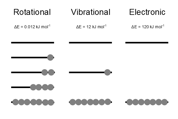
This identification will show the importance of temperature in the Boltzmann distribution. The distribution represents a thermally equilibrated most probable distribution over all energy levels (Figure 17.2.1 ).

The Boltzmann distribution represents a thermally equilibrated most probable distribution over all energy levels. There is always a higher population in a state of lower energy than in one of higher energy.
Once we know the probability distribution for energy, we can calculate thermodynamic properties like the energy, entropy, free energies and heat capacities, which are all average quantities (Equation \(\ref{avg}\)). To calculate \(P_j\), we need the energy levels of a system (i.e., \(\{e_i\}\)). The energy ("levels") of a system can be built up from the quantum energy levels
It must always be remembered that no matter how large the energy spacing is, there is always a non-zero probability of the upper level being populated. The only exception is a system that is at absolute zero. This situation is however hypothetical as absolute zero can be approached but not reached.
Partition Function
The sum over all factors \( e^{-\beta e_j} \) is given a name. It is called the molecular partition function, \(q\):
\[ q = \sum_j e^{-\beta e_j} \nonumber \]
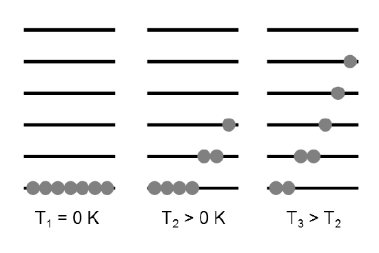
The molecular partition function \(q\) gives an indication of the average number of states that are thermally accessible to a molecule at the temperature of the system. The partition function is a sum over states (of course with the Boltzmann factor \(\beta\) multiplying the energy in the exponent) and is a number. Larger the value of \(q\), larger the number of states which are available for the molecular system to occupy (Figure 17.2.2 ).

We distinguish here between the partition function of the ensemble, \(Q\) and that of an individual molecule, \(q\). Since \(Q\) represents a sum over all states accessible to the system it can written as:
\[ Q(N,V,T) = \sum_{i,j,k ...} e^{-\beta ( e_i + e_j +e_k ...)} \nonumber \]
where the indices \(i,\,j,\,k\) represent energy levels of different particles.
Regardless of the type of particle the molecular partition function, \(q\) represents the energy levels of one individual molecule. We can rewrite the above sum as:
\[Q = q_iq_jq_k… \nonumber \]
or:
\[Q = q^N \nonumber \]
for \(N\) particles. Note that \(q_i\) means a sum over states or energy levels accessible to molecule \(i\) and \(q_j\) means the same for molecule \(j\). The molecular partition function, \(q\) counts the energy levels accessible to molecule \(i\) only. \(Q\) counts not only the states of all of the molecules, but all of the possible combinations of occupations of those states. However, if the particles are not distinguishable then we will have counted \(N!\) states too many. The factor of \(N!\) is exactly how many times we can swap the indices in \(Q(N,V,T)\) and get the same value (again provided that the particles are not distinguishable). See this video for more information.
References
- Hakala, R.W. (1967). Simple justification of the form of Boltzmann's distribution law. Journal of Chemical Education. 44(11), 657. doi: 10.1021/ed044p657
- Grigorenko, I, Garcia, M.E. (2002). Calculation of the partition function using quantum genetic algorithms. Physica A: Satistical Mechanics and its Applications. 313. 463-470. Retrieved from http://www.sciencedirect.com/science...78437102009883
Problems
- Complete the justification of Boltzmann's distribution law by computing the proportionality constant \(a\).
- A system contains two energy levels \(E_1, E_2\). Using Boltzmann statistics, express the average energy of the system in terms of \(E_1, E_2\).
- Consider a system contains N energy levels. Redo problem #2.
- Use the property of exponential function, derive equation (17.9).
- What are the uses of partition functions?

