
4: Electronic and Vibrational States of Crystals
- Page ID
- 474740

\( \newcommand{\vecs}[1]{\overset { \scriptstyle \rightharpoonup} {\mathbf{#1}} } \)
\( \newcommand{\vecd}[1]{\overset{-\!-\!\rightharpoonup}{\vphantom{a}\smash {#1}}} \)
\( \newcommand{\dsum}{\displaystyle\sum\limits} \)
\( \newcommand{\dint}{\displaystyle\int\limits} \)
\( \newcommand{\dlim}{\displaystyle\lim\limits} \)
\( \newcommand{\id}{\mathrm{id}}\) \( \newcommand{\Span}{\mathrm{span}}\)
( \newcommand{\kernel}{\mathrm{null}\,}\) \( \newcommand{\range}{\mathrm{range}\,}\)
\( \newcommand{\RealPart}{\mathrm{Re}}\) \( \newcommand{\ImaginaryPart}{\mathrm{Im}}\)
\( \newcommand{\Argument}{\mathrm{Arg}}\) \( \newcommand{\norm}[1]{\| #1 \|}\)
\( \newcommand{\inner}[2]{\langle #1, #2 \rangle}\)
\( \newcommand{\Span}{\mathrm{span}}\)
\( \newcommand{\id}{\mathrm{id}}\)
\( \newcommand{\Span}{\mathrm{span}}\)
\( \newcommand{\kernel}{\mathrm{null}\,}\)
\( \newcommand{\range}{\mathrm{range}\,}\)
\( \newcommand{\RealPart}{\mathrm{Re}}\)
\( \newcommand{\ImaginaryPart}{\mathrm{Im}}\)
\( \newcommand{\Argument}{\mathrm{Arg}}\)
\( \newcommand{\norm}[1]{\| #1 \|}\)
\( \newcommand{\inner}[2]{\langle #1, #2 \rangle}\)
\( \newcommand{\Span}{\mathrm{span}}\) \( \newcommand{\AA}{\unicode[.8,0]{x212B}}\)
\( \newcommand{\vectorA}[1]{\vec{#1}} % arrow\)
\( \newcommand{\vectorAt}[1]{\vec{\text{#1}}} % arrow\)
\( \newcommand{\vectorB}[1]{\overset { \scriptstyle \rightharpoonup} {\mathbf{#1}} } \)
\( \newcommand{\vectorC}[1]{\textbf{#1}} \)
\( \newcommand{\vectorD}[1]{\overrightarrow{#1}} \)
\( \newcommand{\vectorDt}[1]{\overrightarrow{\text{#1}}} \)
\( \newcommand{\vectE}[1]{\overset{-\!-\!\rightharpoonup}{\vphantom{a}\smash{\mathbf {#1}}}} \)
\( \newcommand{\vecs}[1]{\overset { \scriptstyle \rightharpoonup} {\mathbf{#1}} } \)
\(\newcommand{\longvect}{\overrightarrow}\)
\( \newcommand{\vecd}[1]{\overset{-\!-\!\rightharpoonup}{\vphantom{a}\smash {#1}}} \)
\(\newcommand{\avec}{\mathbf a}\) \(\newcommand{\bvec}{\mathbf b}\) \(\newcommand{\cvec}{\mathbf c}\) \(\newcommand{\dvec}{\mathbf d}\) \(\newcommand{\dtil}{\widetilde{\mathbf d}}\) \(\newcommand{\evec}{\mathbf e}\) \(\newcommand{\fvec}{\mathbf f}\) \(\newcommand{\nvec}{\mathbf n}\) \(\newcommand{\pvec}{\mathbf p}\) \(\newcommand{\qvec}{\mathbf q}\) \(\newcommand{\svec}{\mathbf s}\) \(\newcommand{\tvec}{\mathbf t}\) \(\newcommand{\uvec}{\mathbf u}\) \(\newcommand{\vvec}{\mathbf v}\) \(\newcommand{\wvec}{\mathbf w}\) \(\newcommand{\xvec}{\mathbf x}\) \(\newcommand{\yvec}{\mathbf y}\) \(\newcommand{\zvec}{\mathbf z}\) \(\newcommand{\rvec}{\mathbf r}\) \(\newcommand{\mvec}{\mathbf m}\) \(\newcommand{\zerovec}{\mathbf 0}\) \(\newcommand{\onevec}{\mathbf 1}\) \(\newcommand{\real}{\mathbb R}\) \(\newcommand{\twovec}[2]{\left[\begin{array}{r}#1 \\ #2 \end{array}\right]}\) \(\newcommand{\ctwovec}[2]{\left[\begin{array}{c}#1 \\ #2 \end{array}\right]}\) \(\newcommand{\threevec}[3]{\left[\begin{array}{r}#1 \\ #2 \\ #3 \end{array}\right]}\) \(\newcommand{\cthreevec}[3]{\left[\begin{array}{c}#1 \\ #2 \\ #3 \end{array}\right]}\) \(\newcommand{\fourvec}[4]{\left[\begin{array}{r}#1 \\ #2 \\ #3 \\ #4 \end{array}\right]}\) \(\newcommand{\cfourvec}[4]{\left[\begin{array}{c}#1 \\ #2 \\ #3 \\ #4 \end{array}\right]}\) \(\newcommand{\fivevec}[5]{\left[\begin{array}{r}#1 \\ #2 \\ #3 \\ #4 \\ #5 \\ \end{array}\right]}\) \(\newcommand{\cfivevec}[5]{\left[\begin{array}{c}#1 \\ #2 \\ #3 \\ #4 \\ #5 \\ \end{array}\right]}\) \(\newcommand{\mattwo}[4]{\left[\begin{array}{rr}#1 \amp #2 \\ #3 \amp #4 \\ \end{array}\right]}\) \(\newcommand{\laspan}[1]{\text{Span}\{#1\}}\) \(\newcommand{\bcal}{\cal B}\) \(\newcommand{\ccal}{\cal C}\) \(\newcommand{\scal}{\cal S}\) \(\newcommand{\wcal}{\cal W}\) \(\newcommand{\ecal}{\cal E}\) \(\newcommand{\coords}[2]{\left\{#1\right\}_{#2}}\) \(\newcommand{\gray}[1]{\color{gray}{#1}}\) \(\newcommand{\lgray}[1]{\color{lightgray}{#1}}\) \(\newcommand{\rank}{\operatorname{rank}}\) \(\newcommand{\row}{\text{Row}}\) \(\newcommand{\col}{\text{Col}}\) \(\renewcommand{\row}{\text{Row}}\) \(\newcommand{\nul}{\text{Nul}}\) \(\newcommand{\var}{\text{Var}}\) \(\newcommand{\corr}{\text{corr}}\) \(\newcommand{\len}[1]{\left|#1\right|}\) \(\newcommand{\bbar}{\overline{\bvec}}\) \(\newcommand{\bhat}{\widehat{\bvec}}\) \(\newcommand{\bperp}{\bvec^\perp}\) \(\newcommand{\xhat}{\widehat{\xvec}}\) \(\newcommand{\vhat}{\widehat{\vvec}}\) \(\newcommand{\uhat}{\widehat{\uvec}}\) \(\newcommand{\what}{\widehat{\wvec}}\) \(\newcommand{\Sighat}{\widehat{\Sigma}}\) \(\newcommand{\lt}{<}\) \(\newcommand{\gt}{>}\) \(\newcommand{\amp}{&}\) \(\definecolor{fillinmathshade}{gray}{0.9}\)Schrödinger’s Equation
Electronic and vibrational states describe the characteristics of electronic distributions and atomic oscillations for molecules and solids. Electronic states are wavefunctions \(\Psi_{el}\left( \boldsymbol{r}_{1},\ldots,\boldsymbol{r}_{N};\ \sigma_{1},\ldots,\sigma_{N} \right)\) of the electronic spatial \(\left( \boldsymbol{r}_{i} \right)\) and spin \(\left( \sigma_{i} \right)\) coordinates. Vibrational states are wavefunctions \(\Psi_{vib}\left( \boldsymbol{u}_{1},\ldots,\boldsymbol{u}_{N} \right)\) of small displacements of atoms from their equilibrium positions \(\left( \boldsymbol{u}_{i} = \boldsymbol{R}_{i} - \boldsymbol{R}_{i0} \right)\). These wavefunctions are eigenfunctions of the time-independent Schrödinger equation \(H\Psi = E\Psi\), in which \(H\) is the Hamiltonian (energy operator) consisting of the sum of kinetic and potential energy operators acting on the wavefunction \(\Psi\), and the eigenvalue E is the energy of the state \(\Psi\). For the moment, we focus on electronic states and will briefly address vibrational states later.
Solving the Schrödinger equation for electronic states starts with the Born-Oppenheimer approximation and then involves methods such as Hartree-Fock techniques or density functional theory to address the challenges of electron-electron interactions. Many approaches yield effective one-electron wavefunctions or orbitals \(\psi_{n}\left( \boldsymbol{r} \right)\), which describe the spatial distribution of electrons. When spin-orbit coupling or the presence of any magnetic fields are neglected, electron spin doubles the degeneracy of every orbital. These one-electron wavefunctions are eigenfunctions of the general effective one-electron Schrödinger equation
\[H\left( \boldsymbol{r} \right)\psi_{n}\left( \boldsymbol{r} \right) = \left( T\left( \boldsymbol{r} \right) + V\left( \boldsymbol{r} \right) \right)\psi_{n}\left( \boldsymbol{r} \right) = E_{n}\psi_{n}\left( \boldsymbol{r} \right). \nonumber \]
The energy operator \(H\left( \boldsymbol{r} \right)\) depends on electronic position \(\mathbf{r}\) because expressions for the kinetic energy operator \(T\left( \boldsymbol{r} \right)\) involves spatial second derivatives and the potential energy operator \(V\left( \boldsymbol{r} \right)\) depends on electronic positions relative to the atomic nuclei. The orbitals \(\psi_{n}\left( \boldsymbol{r} \right)\) and their corresponding energies En are labeled by quantum numbers n that depend on the symmetry and boundary conditions associated with the chemical structure. As eigenfunctions of \(H\left( \boldsymbol{r} \right)\), each orbital \(\psi_{n}\left( \boldsymbol{r} \right)\) is normalized and two orbitals with different quantum numbers \(\psi_{m}\left( \boldsymbol{r} \right)\) and \(\psi_{n}\left( \boldsymbol{r} \right)\) are orthogonal:
\[\int_{}^{}{\psi_{m}^{*}\left( \boldsymbol{r} \right)\psi_{n}\left( \boldsymbol{r} \right)dr} \equiv \left\langle \psi_{m} \middle| \psi_{n} \right\rangle = \delta_{mn}, \nonumber \]
where ( \(\delta_{mn}\) = 1 if m = n; \(\delta_{mn}\) = 0 if m ≠ n).
This integral defines the Dirac bra-ket notation. As a result, each eigenvalue is
\[E_{n} = \int_{}^{}{\psi_{n}^{*}\left( \boldsymbol{r} \right)H(\boldsymbol{r})\psi_{n}\left( \boldsymbol{r} \right)dr} \equiv \left\langle \psi_{n} \middle| H \middle| \psi_{n} \right\rangle. \nonumber \]
Moreover, each orbital yields a probability distribution of electron density \(\rho_{n}\left( \boldsymbol{r} \right)\) given as
\[\rho_{n}\left( \boldsymbol{r} \right) = \psi_{n}^{*}\left( \boldsymbol{r} \right)\psi_{n}\left( \boldsymbol{r} \right). \nonumber \]
At this point, how do the symmetry operations of a point group or a space group affect the Schrödinger equation? Since the Schrödinger equation is an equality between two scalar functions, consider how transformations affect scalar functions in general.
Transformations of Scalar Functions
Scalar functions have a definite numerical value \(\varphi(\boldsymbol{r})\) at every point \(\boldsymbol{r}\) in space, and that value is independent of any coordinate system. In a different coordinate system, the point \(\boldsymbol{r}\) will be expressed as \(\boldsymbol{r}'\) and the function will be expressed by \(\varphi'\), but the scalar value \(\varphi'(\boldsymbol{r}')\) remains unchanged, i.e., \(\varphi'(\boldsymbol{r}') = \varphi(\boldsymbol{r})\).
Consider a transformation \(G\) that takes \(\boldsymbol{r}\) to \(\boldsymbol{r}'\), i.e., \(\boldsymbol{r}' = G\boldsymbol{r}\). Then, the function \(\varphi\) transforms into the new function \(\varphi' = G\varphi\), and
\[\varphi'(\boldsymbol{r}') = G\varphi(G\boldsymbol{r}) = \varphi(\boldsymbol{r}) \nonumber \]
or
\[G\varphi(\boldsymbol{r}) = \varphi(G^{- 1}\boldsymbol{r}). \nonumber \]
As a result, the expression for the new function \(\varphi' = G\varphi\) can be determined by evaluating the original function \(\varphi\) at \(G^{- 1}\boldsymbol{r}\).
For \(\varphi(x) = e^{- Zx}\) and \(Gx = x + a\), determine the expression for \(G\varphi(x)\).
Since
\[x = \left( GG^{- 1} \right)x = G\left( G^{- 1}x \right) = G^{- 1}x + a\), then \(G^{- 1}x = x - a. \nonumber \]
Therefore,
\[G\varphi(x) = \varphi\left( G^{- 1}x \right) = \varphi(x - a) = e^{- Z(x - a)}. \nonumber \]
The figure below illustrates this result:
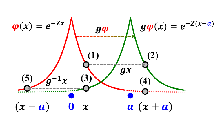
Red Curve: \(\varphi(x) = e^{- Zx}\) around the origin.
Green Curve: \(G\varphi(x) = e^{- Z(x - a)}\) around \(a\).
- \(\varphi(x)\)
- \(G\varphi(Gx) = G\varphi(x + a) = \varphi(x)\)
- \(G\varphi(x) \neq \varphi(x)\)
- \(\varphi(Gx) = \varphi(x + a) \neq \varphi(x)\)
- \(\varphi\left( G^{- 1}x \right) = \varphi(x - a) = G\varphi(x)\)
Now, consider a group of g operations \(\{ E,\ G_{2},\ \ldots,\ G_{g}\}\) such that \(G_{k} = G_{i}G_{j}\). This product operates right-to-left on coordinates, which means \(G_{k}\boldsymbol{r} = G_{i}G_{j}\boldsymbol{r} = G_{i}\left( G_{j}\boldsymbol{r} \right)\). To obtain the same product outcome when applied to functions, the product must operate as follows:
\[G_{k}\varphi\left( \boldsymbol{r} \right) = G_{i}G_{j}\varphi\left( \boldsymbol{r} \right) = G_{i}\left\lbrack G_{j}\varphi\left( \boldsymbol{r} \right) \right\rbrack = G_{j}\varphi\left( G_{i}^{- 1}\boldsymbol{r} \right) = \varphi\left( G_{j}^{- 1}G_{i}^{- 1}\boldsymbol{r} \right) = \varphi\left( {(G_{i}G_{j})}^{- 1}\boldsymbol{r} \right) = \varphi\left( G_{k}^{- 1}\boldsymbol{r} \right) \nonumber \]
Returning to the effective one-electron Schrödinger equation, consider a transformation \(G\) acting on the function \(H\left( \boldsymbol{r} \right)\psi_{n}\left( \boldsymbol{r} \right)\):
\(G\left\lbrack H\left( G\boldsymbol{r} \right)\psi_{n}\left( G\boldsymbol{r} \right) \right\rbrack = GH\left( G\boldsymbol{r} \right)\left\lbrack G^{- 1}\psi_{n}\left( \boldsymbol{r} \right) \right\rbrack = \left\lbrack GH\left( G\boldsymbol{r} \right)G^{- 1} \right\rbrack\psi_{n}\left( \boldsymbol{r} \right) = H\left( \boldsymbol{r} \right)\psi_{n}\left( \boldsymbol{r} \right)\)
If the operation \(G\) is a member of the space group for the crystalline structure being studied, then the one-electron Hamiltonian is invariant with respect to this transformation, i.e., \(H\left( G\mathbf{r} \right) = H\left( \mathbf{r} \right)\). As a result,
\[GH\left( G\mathbf{r} \right)G^{- 1} = GH\left( \mathbf{r} \right)G^{- 1} = H\left( \mathbf{r} \right)\), or \(GH\left( \mathbf{r} \right) = H\left( \mathbf{r} \right)G. \nonumber \]
i.e., \(G\) commutes with \(H\left( \boldsymbol{r} \right)\). The set \(\mathcal{G}\) of all operations \(\{ E,G_{2},\ldots,G_{g}\}\) that commute with \(H\left( \boldsymbol{r} \right)\) forms a group called the group of the Hamiltonian or the group of the Schrödinger equation. These operations do not change the kinetic and potential energy operators. Since the potential energy operator depends on the atomic positions of the structure, then this set contains all operations that keep the structure invariant. Therefore, for a crystalline solid this set is the space group.
So, for \(\psi_{n}\left( \boldsymbol{r} \right)\) an eigenfunction of \(H\left( \boldsymbol{r} \right)\) with eigenvalue En, every transformed wavefunction \(G_{j}\psi_{n}\left( \boldsymbol{r} \right)\) is also an eigenfunction of \(H\left( \boldsymbol{r} \right)\) with the same eigenvalue En. Furthermore, the wavefunction \(\psi_{n}\left( \boldsymbol{r} \right)\) is a basis function for an irreducible representation of the group \(\mathcal{G}\). Now, there are two types of eigenfunctions of the Schrödinger equation to consider:
- \(\psi_{n}\left( \boldsymbol{r} \right)\) is NONDEGENERATE: Given the characteristics of eigenfunctions of the Schrödinger equation, \(G_{j}\psi_{n}\left( \boldsymbol{r} \right)\) will differ from \(\psi_{n}\left( \boldsymbol{r} \right)\) by at most a phase factor1, i.e.,
\[G_{j}\psi_{n}\left( \boldsymbol{r} \right) = \psi_{n}\left( G_{j}^{- 1}\boldsymbol{r} \right) = {e^{i\omega_{j}}\psi}_{n}\left( \boldsymbol{r} \right) \equiv D^{(n)}\left( G_{j} \right)\psi_{n}\left( \boldsymbol{r} \right). \nonumber \]
\(D^{(n)}\left( G_{j} \right) = e^{i\omega_{j}}\) is a 1×1 matrix representative of \(G_{j}\) when \(G_{j}\) operates on the normalized function \(\psi_{n}\left( \boldsymbol{r} \right)\). Applying a second operation \(G_{i}\) to \(G_{j}\psi_{n}\left( \boldsymbol{r} \right)\) yields
\[G_{i}G_{j}\psi_{n}\left( \boldsymbol{r} \right) = {e^{i\omega_{i}}e^{i\omega_{j}}\psi}_{n}\left( \boldsymbol{r} \right) = D^{(n)}\left( G_{i} \right)D^{(n)}\left( G_{j} \right)\psi_{n}\left( \boldsymbol{r} \right). \nonumber \]
If \(G_{i}G_{j} = G_{k}\), then \(D^{(n)}\left( G_{k} \right) = e^{i\omega_{k}} = e^{i\omega_{i}}e^{i\omega_{j}} = D^{(n)}\left( G_{i} \right)D^{(n)}\left( G_{j} \right) = D^{(n)}\left( G_{i}G_{j} \right)\).
Therefore, application of each group operation \(G_{j}\) to \(\psi_{n}\left( \boldsymbol{r} \right)\) creates a 1-dimensional irreducible representation \(D^{(n)}\) of the group of the Hamiltonian \(\mathcal{G}\) with the eigenfunction \(\psi_{n}\left( \boldsymbol{r} \right)\) serving as a basis function. Different nondegenerate eigenfunctions of \(H\left( \boldsymbol{r} \right)\) can be basis functions for the same irreducible representation of the group \(\mathcal{G}\).
- \(\psi_{n}\left( \boldsymbol{r} \right)\) is DEGENERATE: If \(\psi_{n}^{(l)}\left( \boldsymbol{r} \right)\) is one of \(m\) degenerate eigenfunctions \(\psi_{n}^{(p)}\left( \boldsymbol{r} \right)\), \((p = 1,\ldots,m)\), then \(G_{j}\psi_{n}^{(l)}\left( \boldsymbol{r} \right)\) will be a linear combination of the entire set of \(m\) eigenfunctions:
\[G_{j}\psi_{n}^{(l)}\left( \boldsymbol{r} \right) = \sum_{p = 1}^{m}{\left\lbrack D^{(n)}(G_{j}) \right\rbrack_{pl}\psi_{n}^{(p)}\left( \boldsymbol{r} \right)}. \nonumber \]
\(D^{(n)}(G_{j})\) is an \(m \times m\) matrix representative of operation \(G_{j}\) and \(\left\lbrack D^{(n)}(G_{j}) \right\rbrack_{pl}\) is the matrix element of the pth row and the lth column of this matrix. Applying \(G_{i}\) to \(G_{j}\psi_{n}^{(l)}\left( \boldsymbol{r} \right)\) yields
\(G_{i}G_{j}\psi_{n}^{(l)}\left( \boldsymbol{r} \right) = G_{i}\left( \sum_{r = 1}^{m}{\left\lbrack D^{(n)}(G_{j}) \right\rbrack_{rl}\psi_{n}^{(r)}\left( \boldsymbol{r} \right)} \right) = \sum_{r = 1}^{m}{\left\lbrack D^{(n)}(G_{j}) \right\rbrack_{rl}\ G_{i}\psi_{n}^{(r)}\left( \boldsymbol{r} \right)}\) \(R_{i}R_{j}\psi_{n}^{(l)}\left( \boldsymbol{r} \right) = \sum_{r = 1}^{m}{\left\lbrack D^{(n)}(G_{j}) \right\rbrack_{rl}\left( \sum_{p = 1}^{m}{\left\lbrack D^{(n)}(G_{i}) \right\rbrack_{pr}\ \psi_{n}^{(p)}\left( \boldsymbol{r} \right)} \right)}\)
\(R_{i}R_{j}\psi_{n}^{(l)}\left( \boldsymbol{r} \right) = \sum_{r = 1}^{m}{\sum_{p = 1}^{m}{\left\lbrack D^{(n)}(G_{i}) \right\rbrack_{pr}\left\lbrack D^{(n)}(G_{j}) \right\rbrack_{rl}\ \psi_{n}^{(p)}\left( \boldsymbol{r} \right)}}\)
\(R_{i}R_{j}\psi_{n}^{(l)}\left( \boldsymbol{r} \right) = \sum_{p = 1}^{m}{\left( \sum_{r = 1}^{m}{\left\lbrack D^{(n)}(G_{i}) \right\rbrack_{pr}\left\lbrack D^{(n)}(G_{j}) \right\rbrack_{rl}} \right)\psi_{n}^{(p)}\left( \boldsymbol{r} \right)}\)
\[R_{i}R_{j}\psi_{n}^{(l)}\left( \boldsymbol{r} \right) = \sum_{p = 1}^{m}{\left\lbrack D^{(n)}(G_{i}G_{j}) \right\rbrack_{pl}\ \psi_{n}^{(p)}\left( \boldsymbol{r} \right)}. \nonumber \]
If \(G_{i}G_{j} = G_{k}\), then \(D^{(n)}\left( G_{k} \right) = D^{(n)}\left( G_{i}G_{j} \right) = D^{(n)}(G_{i})D^{(n)}(G_{j})\), so that \(D^{(n)}\) is an \(m\)-dimensional representation of the group \(\mathcal{G}\). This representation is irreducible, unless the degeneracy is accidental, which means that not all symmetries of the problem have been properly identified.
(39) We can now make the following assertions regarding the symmetry of the Schrödinger equation for a crystalline solid adopting space group \(\mathcal{G = R}\bigotimes_{}^{}\mathcal{L} = \left\{ \left( R \middle| \boldsymbol{\tau}_{R} \right) \right\}\bigotimes_{}^{}{\ \left\{ \left( 1 \middle| \boldsymbol{T}_{mnp} \right) \right\}}\):
(a) The Hamiltonian \(H(\boldsymbol{r})\) is invariant for all operations of the space group. That is, \(H(\boldsymbol{r})\) is totally symmetric for the space group. Since the operations of the Bravais lattice \(\mathcal{L}\) form a subgroup of \(\mathcal{G}\), then \(H(\boldsymbol{r})\) is also periodic in the Bravais lattice:
\[\left( 1 \middle| \boldsymbol{T}_{mnp} \right)H\left( \boldsymbol{r} \right) = H\left( \left( 1 \middle| \boldsymbol{T}_{mnp} \right)^{- 1}\boldsymbol{r} \right) = H\left( \boldsymbol{r} - \boldsymbol{T}_{mnp} \right) = H\left( \boldsymbol{r} \right). \nonumber \]
By replacing \(\boldsymbol{r}\) with \(\boldsymbol{r} + \boldsymbol{T}_{mnp}\), then
\[H\left( \boldsymbol{r} + \boldsymbol{T}_{mnp} \right) = H\left( \boldsymbol{r} \right). \nonumber \]
(b) The eigenvalues (energies) \(E_{n}\) are invariant for all operations of the space group because they are scalar values. The “quantum numbers” \(n\) serve as labels for the wavefunctions \(\psi_{n}\left( \boldsymbol{r} \right)\).
(c) The eigenfunctions (orbitals) \(\psi_{n}\left( \boldsymbol{r} \right)\) are basis functions for irreducible representations of the space group. Since \(\mathcal{L}\) is an invariant subgroup of \(\mathcal{G}\), these representations can be built (“induced”) from the irreducible representations of the translational symmetry operations \(\mathcal{L}\).
Therefore, before examining the irreducible representations of a space group, we start with irreducible representations of translational symmetry operations \(\mathcal{L}\), which introduces the concept of reciprocal space or k-space.
Representations
Symmetry operations are linear operators that transform sets of coordinates or functions of a vector space into new coordinates or new functions of the same vector space. To evaluate these changes, the symmetry operations are represented by square matrices, for which the number of rows or columns is the dimension of the representation. Since there are many possible vector spaces that can be used to describe atomic and electronic structure, there are several possible representations of symmetry groups. Most representations are reducible, which means that every matrix can be written in an equivalent block-diagonal form after a similarity transformation:2
\[D(R) = \begin{pmatrix} D^{(1)}(R) & 0 & \cdots & 0 \\ 0 & D^{(2)}(R) & \cdots & 0 \\ \vdots & \vdots & \ddots & \vdots \\ 0 & 0 & \cdots & D^{(\mu)}(R) \\ \end{pmatrix} \equiv D^{(1)}(R)\bigoplus_{}^{}{D^{(2)}(R)}\bigoplus_{}^{}{\cdots\bigoplus_{}^{}{D^{(\mu)}(R)}}. \nonumber \]
If a matrix representation cannot be transformed into block-diagonal form, then the representation is called irreducible. Irreducible representations (IRs) are the fundamental representations from which all reducible representations for a group can be composed. One-dimensional representations are scalars, and are necessarily irreducible. There are 1-, 2-, and 3-dimensional IRs among the crystallographic point groups, and the non-crystallographic icosahedral point groups \(\mathcal{I}\) and \(\mathcal{I}_{h}\) allow 4- and 5-dimensional IRs.
GREAT ORTHOGONALITY THEOREM (“GOT”)
If \(D^{(i)}\) and \(D^{(j)}\) are two irreducible representations of a group \(\mathcal{G}\), then this theorem provides the following relationships among the matrix elements of these two representations:
\[\sum_{R \in \mathcal{G}}^{}{\left\lbrack D^{(i)}(R) \right\rbrack_{\mu\nu}^{*}\ \left\lbrack D^{(j)}(R) \right\rbrack_{\mu'\nu'}} = \frac{g}{l_{i}}\ \delta_{ij}\ \delta_{\mu\mu'}\ \delta_{\nu\nu'}. \nonumber \]
In this equation, \(\left\lbrack D^{(i)}(R) \right\rbrack_{\mu\nu}\) is the matrix element of the \(\mu\)th row and \(\nu\)th column of the matrix representative \(D^{(i)}\) for the operation \(R\) of \(\mathcal{G}\). The dimension of \(D^{(i)}\) is \(l_{i}\). Given the equivalence of representations related to each other by a similarity transformation, this theorem can be revised to express relationships among the characters \(\chi^{(i)}(R)\) of IRs. Recall, the character of a representation for a specific group member is the trace of the corresponding matrix. Because the character is invariant under any similarity transformation, operations belonging to the same class of a group have the same character. Also, the dimension of a representation is the character of the identity operation. From the GOT, several important relationships involving characters can be deduced:
- Two equivalent representations have equal sets of characters;
- A representation is irreducible if and only if \(\sum_{R \in \mathcal{G}}^{}\left| \chi(R) \right|^{2} = g\);
- The number of times \(n_{i}\) that IR \(D^{(i)}\) occurs in the reduction of a reducible representation \(D\) is \(n_{i} = \frac{1}{g}\sum_{R \in \mathcal{G}}^{}{\ \chi(R){\chi^{(i)}(R)}^{*}}\);
- The number of IRs equals the number of classes in a group;
- The order of the group equals the sum of the squared dimensions of all IRs: \(g = \sum_{}^{}l_{i}^{2}\);
- The sum of characters of the entire group for different IRs are orthogonal: \(\sum_{R \in \mathcal{G}}^{}{{\chi^{(i)}(R)}^{*}\chi^{(j)}(R)} = g\delta_{ij}\);
- The sum of characters for different classes over all IRs are orthogonal: \(\sum_{i}^{}{\chi^{(i)}\left( \mathcal{C}_{k} \right)}^{*}\chi^{(i)}\left( \mathcal{C}_{j} \right)N_{k} = g\delta_{kj}\), in which the sum is over all IRs and \(N_{k} =\) number of members in class \(\mathcal{C}_{k}\).
The last four relationships provide the basis for constructing character tables for finite groups:
| \mathcal{G} | \mathcal{C}_{1} = E | \cdots | \mathcal{C}_{k} | \cdots | \mathcal{C}_{N} | Basis Function(s) |
|---|---|---|---|---|---|---|
| IR D^{(1)} | 1 | \cdots | 1 | \cdots | 1 | \psi_{1} (1-d; Totally Symmetric IR) |
| \vdots | \vdots | \vdots | \ \vdots | |||
| IR D^{(i)} | l_{i} | \cdots | \chi^{(i)}\left( \mathcal{C}_{k} \right) | \cdots | \chi^{(i)}\left( \mathcal{C}_{N} \right) | \psi_{i} |
| \vdots | \vdots | \vdots | \ \vdots | |||
| IR D^{(N)} | l_{N} | \cdots | \chi^{(N)}\left( \mathcal{C}_{k} \right) | \cdots | \chi^{(N)}\left( \mathcal{C}_{N} \right) | \psi_{N} |
RECIPROCAL SPACE
Periodic Functions on a Lattice
If \(\psi(x)\) has the total symmetry of a 1-d Bravais lattice with distance \(a\) between adjacent lattice points, then
\[\psi(x + ma) = \psi(x) \nonumber \]
for all integers \(m\)? Naturally periodic functions include transcendental functions like \(A\sin{kx}\) and \(A\cos{kx}\) in which the wavevector \(k\) is related to the wavelength \(\lambda\) by \(k = \frac{2\pi}{\lambda}\). As a specific example, for any general value of \(k\), the function \(A\cos{kx}\) is not periodic with respect to this lattice, as seen to the right. However, for certain values of \(k = K_{h}\), \(A\cos{K_{h}x}\) is periodic with the lattice. The allowed values of \(K_{h}\) are determined by equating \(\psi(x + a)\) with \(\psi(x)\) because \(a\) represents the smallest repeating distance of the lattice:
\[A\cos{K_{h}(x + a)} = A\cos{K_{h}x} = A\cos{K_{h}x}\cos{K_{h}a} - A\sin{K_{h}x}\sin{K_{h}a}. \nonumber \]

Since \(\cos{kx}\) and \(\sin{kx}\) are, respectively, even and odd functions with respect to inversion through the origin, the term \(A\sin{K_{h}x}\sin{K_{h}a}\) must be eliminated, which means
\[\sin{K_{h}a} = 0 \nonumber \]
or
\[K_{h}a = 2\pi h \nonumber \]
for \(h\) = any integer.
As a result, the values of \(K_{h}\) for which \(A\cos{K_{h}x}\) is periodic on the 1-d lattice with spacing \(a\) between adjacent lattice points are
\[K_{h} = \cdots\frac{- 6\pi}{a},\frac{- 4\pi}{a},\frac{- 2\pi}{a},0,\frac{2\pi}{a},\frac{4\pi}{a},\frac{6\pi}{a},\cdots, \nonumber \]
as the following graphs illustrate for \(K_{h} = \frac{2\pi}{a}\) and \(\frac{- 4\pi}{a}\):
\[\psi(x) = A\cos\frac{2\pi x}{a} \nonumber \]

\[\psi(x) = A\cos\frac{- 4\pi x}{a} \nonumber \]

Both functions are, indeed, periodic on the lattice, but only the function \(A \cos \left( \frac{2 \pi x}{a} \right)\)repeats exactly by the lattice constant \(a\). Among the other solutions, the resulting “wave” for \(K_{h} = 0\) is a constant \(\psi(x) = A\), while the others repeat by integer fractions of \(a\), i.e., \(\frac{a}{h}\). Furthermore, the restriction for the allowed values of \(K_{h}\) also applies to \(A\sin{K_{h}x}\) and the complex plane wave \(Ae^{iK_{h}x} = A\left( \cos{K_{h}x} + i\sin{K_{h}x} \right)\).
\[\sum_{h}{A_{h}\cos{K_{h}x}} \nonumber \]

The most general periodic functions with respect to a 1-d lattice are Fourier series, i.e., sums of cosine and sine functions over all integers \(h\):
\[\sum_{h}^{}{A_{h}\cos{K_{h}x} + B_{h}\sin{K_{h}x}}\ or\ \sum_{h}^{}{C_{h}e^{iK_{h}x}}. \nonumber \]
The infinite sums are truncated, which introduces oscillations in the final function, as shown to the right.
The Reciprocal Lattice
The analysis of periodic functions on a 1-d Bravais lattice in real space, which is the set of points \(\left\{ \cdots, - 2a, - a,0,a,2a,\cdots \right\}\), identifies a lattice in reciprocal space, which is the corresponding set of points \(\left\{ \cdots,\frac{- 4\pi}{a},\frac{- 2\pi}{a},0,\frac{2\pi}{a},\frac{4\pi}{a},\cdots \right\}\).

The reciprocal lattice is the set of all wavevectors, with units (length)–1, that yield plane waves with the periodicity of the Bravais lattice.
For 3-d space, plane wave functions \(\ \psi\left( \boldsymbol{r} \right)\) that have the total symmetry of the 3-d Bravais lattice must obey the following equation:
\[\psi\left( \boldsymbol{r} + \boldsymbol{T}_{mnp} \right) = \psi\left( \boldsymbol{r} \right) = Ae^{i\boldsymbol{K}_{hkl} \cdot \boldsymbol{r}} = Ae^{i\boldsymbol{K}_{hkl} \cdot \left( \boldsymbol{r} + \boldsymbol{T}_{mnp} \right)} = Ae^{i\boldsymbol{K}_{hkl} \cdot \boldsymbol{r}}Ae^{i\boldsymbol{K}_{hkl} \cdot \boldsymbol{T}_{mnp}}. \nonumber \]
which gives the conditions for the reciprocal lattice \(\boldsymbol{K}_{hkl}\):
\[e^{i\boldsymbol{K}_{hkl} \cdot \boldsymbol{T}_{mnp}} = 1 \nonumber \]
or
\[\boldsymbol{K}_{hkl} \cdot \boldsymbol{T}_{mnp} = 2\pi \times \text{integer}. \nonumber \]
To ensure that all reciprocal lattice points are identified, Bravais lattice vectors must be expressed using the primitive cell, i.e., \(\boldsymbol{T}_{mnp} = m\boldsymbol{a}_{1} + n\boldsymbol{a}_{2} + p\boldsymbol{a}_{3};\ m,n,p =\) all integers. Then, the conditions on \(\boldsymbol{K}_{hkl}\) become
- \(\boldsymbol{K}_{hkl} \cdot \boldsymbol{a}_{1} = 2\pi h\)
- \(\boldsymbol{K}_{hkl} \cdot \boldsymbol{a}_{2} = 2\pi k\)
- \(\boldsymbol{K}_{hkl} \cdot \boldsymbol{a}_{3} = 2\pi l\)
- \(h,k,l =\) all integers.
If every reciprocal lattice vector is expressed using its own primitive cell, i.e., \(\boldsymbol{K}_{hkl} = h\boldsymbol{a}_{1}^{*} + k\boldsymbol{a}_{2}^{*} + l\boldsymbol{a}_{3}^{*};\ h,k,l =\) all integers, then the conditions defining the reciprocal lattice become
\[\boldsymbol{a}_{i} \cdot \boldsymbol{a}_{j}^{*} = 2\pi\delta_{ij};\ (i,j = 1,2,3). \nonumber \]
As a result, the primitive unit cell of the Bravais lattice in real space defines the primitive unit cell of the corresponding reciprocal lattice. The 1-d Bravais lattice is \(\left\{ \boldsymbol{T}_{m} = m\boldsymbol{a} \right\}\), the corresponding reciprocal lattice is \(\left\{ \boldsymbol{K}_{h} = h\boldsymbol{a}^{*} \right\}\), and the length of \(\boldsymbol{a}^{*}\) is \(\frac{2\pi}{a}\).
To summarize the results above, once a primitive unit cell in real space is identified, then the corresponding primitive cell of the reciprocal lattice can be calculated:
- Bravais Lattice: \(\left\{ \boldsymbol{T}_{mnp} = m\boldsymbol{a}_{1} + n\boldsymbol{a}_{2} + p\boldsymbol{a}_{3};\ (m,n,p\ \text{integers}) \right\}\)
- Reciprocal Lattice: \(\left\{ \boldsymbol{K}_{hk} = h\boldsymbol{a}_{1}^{*} + k\boldsymbol{a}_{2}^{*} + l\boldsymbol{a}_{3}^{*};\ \left( h,k,l\ \text{integers\ and}\ \boldsymbol{a}_{i} \cdot \boldsymbol{a}_{j}^{*} = 2\pi\delta_{ij} \right) \right\}\).
The conditions relating real space and reciprocal space primitive cell vectors means that \(\boldsymbol{a}_{1}^{*}\) is perpendicular to \(\boldsymbol{a}_{2}\) and \(\boldsymbol{a}_{3}\), \(\boldsymbol{a}_{2}^{*}\) is perpendicular to \(\boldsymbol{a}_{1}\) and \(\boldsymbol{a}_{3}\), and \(\boldsymbol{a}_{3}^{*}\) is perpendicular to \(\boldsymbol{a}_{1}\) and \(\boldsymbol{a}_{2}\). According to these relationships, the primitive vectors of the reciprocal lattice can be determined from the primitive vectors of the real-space Bravais lattice as follows:
\[\boldsymbol{a}_{1}^{*} = 2\pi\frac{\boldsymbol{a}_{2} \times \boldsymbol{a}_{3}}{\boldsymbol{a}_{1} \cdot \boldsymbol{a}_{2} \times \boldsymbol{a}_{3}};\ \ \ \ \ \boldsymbol{a}_{2}^{*} = 2\pi\frac{\boldsymbol{a}_{3} \times \boldsymbol{a}_{1}}{\boldsymbol{a}_{1} \cdot \boldsymbol{a}_{2} \times \boldsymbol{a}_{3}};\ \ \ \ \ \boldsymbol{a}_{3}^{*} = 2\pi\frac{\boldsymbol{a}_{1} \times \boldsymbol{a}_{2}}{\boldsymbol{a}_{1} \cdot \boldsymbol{a}_{2} \times \boldsymbol{a}_{3}}\ . \nonumber \]
The numerators in each equation yield vectors that are orthogonal to the plane of the two vectors; the denominators are all the same and equal the volume of the primitive unit cell \(V_{1}\). Therefore,
\[\boldsymbol{a}_{1}^{*} = 2\pi\frac{\boldsymbol{a}_{2} \times \boldsymbol{a}_{3}}{V_{1}} \nonumber \]
\[\boldsymbol{a}_{2}^{*} = 2\pi\frac{\boldsymbol{a}_{3} \times \boldsymbol{a}_{1}}{V_{1}} \nonumber \]
\[\boldsymbol{a}_{3}^{*} = 2\pi\frac{\boldsymbol{a}_{1} \times \boldsymbol{a}_{2}}{V_{1}}. \nonumber \]
VECTOR PRODUCTS
The expressions defining the primitive cell vectors of the reciprocal lattice use three important vector products, which are described below. In the following, vectors are denoted using boldface.
\(\boldsymbol{a} = a_{x}\widehat{\boldsymbol{x}} + a_{y}\widehat{\boldsymbol{y}} + a_{z}\widehat{\boldsymbol{z}}\) (length \(a\)), \(\boldsymbol{\ b} = b_{x}\widehat{\boldsymbol{x}} + b_{y}\widehat{\boldsymbol{y}} + b_{z}\widehat{\boldsymbol{z}}\) (length \(b\)), and \(\boldsymbol{c} = c_{x}\widehat{\boldsymbol{x}} + c_{y}\widehat{\boldsymbol{y}} + c_{z}\widehat{\boldsymbol{z}}\) (length \(c\)). Vectors with the carrot overhead, such as \(\widehat{\boldsymbol{x}}\), have unit length.
Vector Dot (Scalar) Product of \(\boldsymbol{a}\) and \(\boldsymbol{b}\):
\[\boldsymbol{a} \cdot \boldsymbol{b} = a_{x}b_{x} + a_{y}b_{y} + a_{z}b_{z} = ab\cos\gamma\); \(\gamma =\) angle between \(\boldsymbol{a}\) and \(\boldsymbol{b}. \nonumber \]
Vector Cross Product of \(\boldsymbol{a}\) and \(\boldsymbol{b}\):
\(\boldsymbol{a} \times \boldsymbol{b} = \det\begin{pmatrix} \widehat{\boldsymbol{x}} & \widehat{\boldsymbol{y}} & \widehat{\boldsymbol{z}} \\ a_{x} & a_{y} & a_{z} \\ b_{x} & b_{y} & b_{z} \\ \end{pmatrix} = \left( a_{y}b_{z} - a_{z}b_{y} \right)\widehat{\boldsymbol{x}} + \left( a_{z}b_{x} - a_{x}b_{z} \right)\widehat{\boldsymbol{y}} + \left( a_{x}b_{y} - a_{y}b_{x} \right)\widehat{\boldsymbol{z}}.\)
The length of \(\boldsymbol{a} \times \boldsymbol{b}\) is \(ab\sin\gamma\), \(\gamma =\) angle between \(\boldsymbol{a}\) and \(\boldsymbol{b}\); the orientation of \(\boldsymbol{a} \times \boldsymbol{b}\) is perpendicular to the plane of \(\boldsymbol{a}\) and \(\boldsymbol{b}\) and directed according to the right-hand rule (using your right hand, if the direction of your index finger is the first vector \(\boldsymbol{a}\) and your other fingers curl toward the direction of the second vector \(\boldsymbol{b}\), then the direction of your outstretched thumb is the direction of \(\boldsymbol{a} \times \boldsymbol{b}\)). The length of \(\boldsymbol{a} \times \boldsymbol{b}\) is the area of the parallelogram formed by \(\boldsymbol{a}\) and \(\boldsymbol{b}\).
Vector Triple Product of \(\boldsymbol{a}\), \(\boldsymbol{b}\), and \(\boldsymbol{c}\):
\(\boldsymbol{a} \cdot \boldsymbol{b} \times \boldsymbol{c} = \det\begin{pmatrix} a_{x} & a_{y} & a_{z} \\ b_{x} & b_{y} & b_{z} \\ c_{x} & c_{y} & c_{z} \\ \end{pmatrix} = a_{x}\left( b_{y}c_{z} - b_{z}c_{y} \right) + a_{y}\left( b_{z}c_{x} - b_{x}c_{z} \right) + a_{z}\left( b_{x}c_{y} - b_{y}c_{x} \right).\)
This scalar quantity is the volume of the parallelepiped formed by vectors \(\boldsymbol{a}\), \(\boldsymbol{b}\), and \(\boldsymbol{c}\).
Using these formulas for determining primitive cell vectors for a reciprocal lattice, below are illustrated the reciprocal lattices for each of the five 2-d lattices (to accomplish the vector cross-product, choose \(\boldsymbol{a}_{3}\) to be a unit vector oriented perpendicular to the 2-d Bravais lattice).
@ >p(- 12) * >p(- 12) * >p(- 12) * >p(- 12) * >p(- 12) * >p(- 12) * >p(- 12) * @
() &
() () &
() OBLIQUE: &
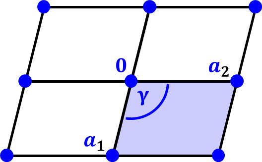
Figure 4.7
\(a_{1} < a_{2}\) & & \(a_{1}^{*} = \frac{2\pi}{a_{1}\sin\gamma}\)
\(a_{2}^{*} = \frac{2\pi}{a_{2}\sin\gamma}\)
\(\gamma^{*} = 180{^\circ} - \gamma\) & & &
RECTANGULAR: & &

Figure 4.9
\(a_{1} < a_{2}\) & & \(a_{1}^{*} = \frac{2\pi}{a_{1}}\)
\(a_{2}^{*} = \frac{2\pi}{a_{2}}\)
\(\gamma^{*} = 90{^\circ}\) & & &
CENTERED RECTANGULAR: & & & & &

Figure 4.11
\(a_{1} = a_{2} = a\) & & \(a_{1}^{*} = \frac{2\pi}{a\sin\gamma}\)
\(a_{2}^{*} = \frac{2\pi}{a\sin\gamma}\)
\(\gamma^{*} = 180{^\circ} - \gamma\) & & &
TETRAGONAL: & &
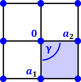
Figure 4.13
\(a_{1} = a_{2} = a\) & & \(a_{1}^{*} = \frac{2\pi}{a}\)
\(a_{2}^{*} = \frac{2\pi}{a}\)
\(\gamma^{*} = 90{^\circ}\) & & &
TRIGONAL/HEXAGONAL: & & &

Figure 4.15
\(a_{1} = a_{2} = a\) & & \(a_{1}^{*} = \frac{2\pi}{a\sin{120{^\circ}}} = \frac{4\pi}{\sqrt{3}a}\)
\(a_{2}^{*} = \frac{2\pi}{a\sin{120{^\circ}}} = \frac{4\pi}{\sqrt{3}a}\)
\(\gamma^{*} = 60{^\circ}\) & & &
()
Some conclusions inferred from these illustrations include:
- The rotational symmetry of the reciprocal lattice matches the rotational symmetry of the Bravais lattice. This is particularly emphasized by the gray-shaded hexagonal regions for the trigonal/hexagonal real space and reciprocal space lattices.
- The relative lengths of the primitive cell parameters of the reciprocal lattice are inversely related to the primitive cell parameters of the real space Bravais lattice.
- The reciprocal lattice for the centered rectangular Bravais lattice is also centered rectangular, but it must be calculated from the primitive unit cell.
In 3-d, the following relationships between real space Bravais lattices and reciprocal lattices hold:
- Primitive real space lattices give primitive reciprocal lattices;
- Base-centered ( \(C\)- or \(A\)-) real space lattices give base-centered reciprocal lattices;
- Body-centered ( \(I\)-) real space lattices give face-centered ( \(F\)-) reciprocal lattices; and
- Face-centered ( \(F\)-) real space lattices give body-centered ( \(I\)-) reciprocal lattices.
The reciprocal lattice for a crystalline solid can be “observed” by diffraction experiments because the condition for constructive interference of diffracted radiation puts the observed diffracted waves at the positions of the reciprocal lattice. Each observable diffraction peak is labeled by its Miller indices (hkl).
Determine the reciprocal lattice for a body-centered cubic real space Bravais lattice with cubic unit cell length \(a\).
- Answer
-
The body-centered cubic cell is \(\boldsymbol{a} = a\widehat{\boldsymbol{x}};\ \ \boldsymbol{b} = a\widehat{\boldsymbol{y}};\ \ \boldsymbol{c} = a\widehat{\boldsymbol{z}}.\) With lattice points at the corners and center of this cell, the primitive unit cell is
\[\boldsymbol{a}_{1} = \frac{a}{2}\widehat{\boldsymbol{x}} - \frac{a}{2}\widehat{\boldsymbol{y}}\boldsymbol{+}\frac{a}{2}\widehat{\boldsymbol{z}};\ \ \boldsymbol{a}_{2} = \frac{a}{2}\widehat{\boldsymbol{x}} + \frac{a}{2}\widehat{\boldsymbol{y}}\boldsymbol{-}\frac{a}{2}\widehat{\boldsymbol{z}};\ \ \boldsymbol{a}_{3} = - \frac{a}{2}\widehat{\boldsymbol{x}} + \frac{a}{2}\widehat{\boldsymbol{y}}\boldsymbol{+}\frac{a}{2}\widehat{\boldsymbol{z}}\boldsymbol{\ }. \nonumber \]
The volume of the primitive cell is \(V_{1} = \frac{a^{3}}{2}\). Then, using the formulas for the primitive cell vectors of the reciprocal lattice, we obtain
\[\small{\boldsymbol{a}_{1}^{*} = \frac{4\pi}{a^{3}}\left\lbrack \frac{a}{2}\left( \widehat{\boldsymbol{x}} + \widehat{\boldsymbol{y}}\boldsymbol{-}\widehat{\boldsymbol{z}} \right) \right\rbrack \times \left\lbrack \frac{a}{2}\left( - \widehat{\boldsymbol{x}} + \widehat{\boldsymbol{y}}\boldsymbol{+}\widehat{\boldsymbol{z}} \right) \right\rbrack = \frac{\pi}{a}\left\lbrack 2\left( \widehat{\boldsymbol{y}}\boldsymbol{\times}\widehat{\boldsymbol{z}} \right) + 2\left( \widehat{\boldsymbol{x}}\boldsymbol{\times}\widehat{\boldsymbol{y}} \right) \right\rbrack = \frac{2\pi}{a}\widehat{\boldsymbol{x}} + \frac{2\pi}{a}\widehat{\boldsymbol{z}}\ ;} \nonumber \]
\[\small{\boldsymbol{a}_{2}^{*} = \frac{4\pi}{a^{3}}\left\lbrack \frac{a}{2}\left( - \widehat{\boldsymbol{x}} + \widehat{\boldsymbol{y}}\boldsymbol{+}\widehat{\boldsymbol{z}} \right) \right\rbrack \times \left\lbrack \frac{a}{2}\left( \widehat{\boldsymbol{x}} - \widehat{\boldsymbol{y}}\boldsymbol{+}\widehat{\boldsymbol{z}} \right) \right\rbrack = \frac{\pi}{a}\left\lbrack 2\left( \widehat{\boldsymbol{y}}\boldsymbol{\times}\widehat{\boldsymbol{z}} \right) + 2\left( \widehat{\boldsymbol{z}}\boldsymbol{\times}\widehat{\boldsymbol{x}} \right) \right\rbrack = \frac{2\pi}{a}\widehat{\boldsymbol{x}} + \frac{2\pi}{a}\widehat{\boldsymbol{y}}\ ;} \nonumber \]
\[\small{\boldsymbol{a}_{3}^{*} = \frac{4\pi}{a^{3}}\left\lbrack \frac{a}{2}\left( \widehat{\boldsymbol{x}} - \widehat{\boldsymbol{y}}\boldsymbol{+}\widehat{\boldsymbol{z}} \right) \right\rbrack \times \left\lbrack \frac{a}{2}\left( \widehat{\boldsymbol{x}} + \widehat{\boldsymbol{y}}\boldsymbol{-}\widehat{\boldsymbol{z}} \right) \right\rbrack = \frac{\pi}{a}\left\lbrack 2\left( \widehat{\boldsymbol{z}}\boldsymbol{\times}\widehat{\boldsymbol{x}} \right) + 2\left( \widehat{\boldsymbol{x}}\boldsymbol{\times}\widehat{\boldsymbol{y}} \right) \right\rbrack = \frac{2\pi}{a}\widehat{\boldsymbol{y}} + \frac{2\pi}{a}\widehat{\boldsymbol{z}}\ .} \nonumber \]
These vectors form the primitive cell for a face-centered cubic lattice. The side of the cubic cell is \(\frac{4\pi}{a}\).

Figure 4.17 The reciprocal lattice partitions reciprocal space into cells and identifies those wavevectors that create plane waves that are periodic with the real space Bravais lattice. Now, what significance do the wavevectors in the region between reciprocal lattice points have?
Irreducible Representations of the 1-d Translation Group
The group of translations in one-dimension is a quasi-infinite set of lattice translations \(\mathcal{L =}\left\{ \left( 1 \middle| \boldsymbol{T}_{m} \right),\ m = integer \right\}\). To make the problem tractable, periodic boundary conditions are applied to this set so that for any vector \(\boldsymbol{x}\), \(\boldsymbol{x} + \boldsymbol{T}_{N} = \boldsymbol{x}\), i.e., \(\boldsymbol{T}_{N}\) is equivalent to the identity translation \(\boldsymbol{T}_{N} = \mathbf{0}\). Since this group of translations is Abelian, each member is its own class and the number of irreducible representations (IRs) equals the number of members of the group. Therefore, each IR is one-dimensional.
As a concrete example, consider a 1-d lattice with lattice constant a and set the periodic boundary condition to be four primitive translations, i.e., \(\boldsymbol{\ }\boldsymbol{T}_{4} = \mathbf{0}\). Let \(\boldsymbol{T}_{m} \equiv \left( 1 \middle| m\boldsymbol{a} \right)\). Then, the set of translation operations that set the Bravais lattice contains 4 members:
\[\mathcal{L =}\left\{ \boldsymbol{T}_{1}\mathbf{,\ }\boldsymbol{T}_{2}\mathbf{,}\boldsymbol{T}_{3}\mathbf{,}\boldsymbol{T}_{4}\mathbf{=}\boldsymbol{T}_{0} \right\} \equiv \left\{ \left( 1 \middle| \boldsymbol{a} \right),\left( 1 \middle| 2\boldsymbol{a} \right),\left( 1 \middle| 3\boldsymbol{a} \right),\left( 1 \middle| 4\boldsymbol{a} \right) = \left( 1 \middle| \mathbf{0} \right) \right\}. \nonumber \]
Therefore, the group has 4 classes and, as a result, 4 1-dimensional IRs, which we can label as \(\mathbf{\Gamma}^{(1)}\), \(\mathbf{\Gamma}^{(2)}\), \(\mathbf{\Gamma}^{(3)}\), and \(\mathbf{\Gamma}^{(4)}\). Therefore, for each class of symmetry operations, the matrix representatives, which are also the characters of these IRs, must be complex numbers.
We use the properties of the group \(\mathcal{L}\) to determine the expressions for these characters. Start by determining the characters of each IR for the fundamental translation \(\boldsymbol{T}_{1} \equiv \left( 1 \middle| \boldsymbol{a} \right)\). Let \(\mathbf{\Gamma}^{(\mu)}\left( \boldsymbol{T}_{1} \right) = \varepsilon_{\mathbf{\mu}}\). If the operation \(\boldsymbol{T}_{1}\) is performed 4 successive times, i.e.,
\({\boldsymbol{T}_{1}}^{4} = \left( 1 \middle| \boldsymbol{a} \right)^{4} = \left( 1 \middle| 4\boldsymbol{a} \right) \equiv \left( 1 \middle| \mathbf{0} \right) = \boldsymbol{T}_{0}\), the identity,
then \({\varepsilon_{\mu}}^{4} = 1\), which has the solutions \(\varepsilon_{\mu} = e^{\frac{- 2\pi i\mu}{4}}\) for \(\mu = 1,\ 2,\ 3,\ 4\):
\[\varepsilon_{1} = e^{\frac{- 2\pi i(1)}{4}} = e^{\frac{- i\pi}{2}} = - i\); \(\varepsilon_{2} = e^{\frac{- 2\pi i(2)}{4}} = e^{- i\pi} = - 1. \nonumber \]
\[\varepsilon_{3} = e^{\frac{- 2\pi i(3)}{4}} = e^{\frac{- 3i\pi}{2}} = + i\); \(\varepsilon_{4} = e^{\frac{- 2\pi i(4)}{4}} = e^{- 2i\pi} = + 1. \nonumber \]
We can use these characters to determine the characters for \(\mathbf{\Gamma}^{(\mu)}\left( \boldsymbol{T}_{m} \right)\):
\(\mathbf{\Gamma}^{(\mu)}\left( \boldsymbol{T}_{m} \right) = \mathbf{\Gamma}^{(\mu)}\left( m\boldsymbol{T}_{1} \right) = \left\lbrack \mathbf{\Gamma}^{(\mu)}\left( \boldsymbol{T}_{1} \right) \right\rbrack^{m} = {\varepsilon_{\mu}}^{m} = e^{\frac{- 2\pi im\mu}{4}}.\)
Therefore, the character or representative of \(\mathbf{\Gamma}^{(\mu)}\left( \boldsymbol{T}_{m} \right)\) contains a label for the class (m) and for the IR ( \(\mu\)). Although this is a convenient formula, it is helpful and useful to relate this expression directly to the lattice vectors \(\boldsymbol{T}_{m}\) rather than just the index \(m\) of the lattice vector. To accomplish this, we rewrite the exponent and do a fair amount of rearrangement:
\[\frac{2\pi im\mu}{4} \cdot \frac{a}{a} = i\left( \frac{2\pi\mu}{4a} \right)(ma) = i\left\lbrack \frac{\mu}{4}\left( \frac{2\pi}{a} \right) \right\rbrack(ma) = i\boldsymbol{k}_{\mu} \cdot \boldsymbol{T}_{m}. \nonumber \]
In this rearrangement of the exponent, \(\boldsymbol{k}_{\mu}\) is the wavevector or k-point associated with the IR \(\mathbf{\Gamma}^{(\mu)}\) of the Bravais lattice group \(\mathcal{\ L}\). Therefore, the character or representative of the IR \(\mathbf{\Gamma}^{(\mu)}\left( \boldsymbol{T}_{m} \right)\) for the lattice translation \(\boldsymbol{T}_{m} = \left( 1 \middle| ma \right)\) is
\[\mathbf{\Gamma}^{(\mu)}\left( \boldsymbol{T}_{m} \right) = e^{- i\boldsymbol{k}_{\mu} \cdot \boldsymbol{T}_{m}}\) = \(\ e^{- 2\pi im\mu/4};\ \ m,\mu = 1,\ 2,\ 3,\ 4. \nonumber \]
in which \(m\) is a class label and \(\mu\) is an IR label.
This equation provides the means to construct the character table for this 1-d translation group. According to the periodic boundary condition \(\boldsymbol{T}_{4} \equiv \left( 1 \middle| 4a \right) = \left( 1 \middle| 0 \right) \equiv \boldsymbol{T}_{0}\), there are 4 classes and, therefore, 4 irreducible representations, which are described by their wavevectors \(\boldsymbol{k}_{\mu}\):
@ >p(- 16) * >p(- 16) * >p(- 16) * >p(- 16) * >p(- 16) * >p(- 16) * >p(- 16) * >p(- 16) * >p(- 16) * @
() &
\[\boldsymbol{T}_{0} \nonumber \]
&
\[\boldsymbol{T}_{1} \nonumber \]
&
\[\boldsymbol{T}_{2} \nonumber \]
&
\[\boldsymbol{T}_{3} \nonumber \]
&
&
() () &
\[\boldsymbol{T}_{0} \nonumber \]
&
\[\boldsymbol{T}_{1} \nonumber \]
&
\[\boldsymbol{T}_{2} \nonumber \]
&
\[\boldsymbol{T}_{3} \nonumber \]
&
&
() & Real & Imaginary & & & & & &
\(k_{1} = \frac{\pi}{2a}\) & \(\mathbf{\Gamma}^{(1)}\) & 1 & –i & –1 & i & \(\varphi_{1}\) & 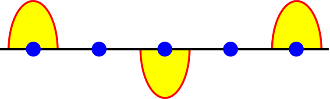
Figure 4.18 & 
Figure 4.19
\(k_{2} = \frac{\pi}{a}\) & \(\mathbf{\Gamma}^{(2)}\) & 1 & –1 & 1 & –1 & \(\varphi_{2}\) & 
Figure 4.20 & 
Figure 4.21
\(k_{3} = \frac{3\pi}{2a}\) & \(\mathbf{\Gamma}^{(3)}\) & 1 & i & –1 & –i & \(\varphi_{3}\) & 
Figure 4.22 & 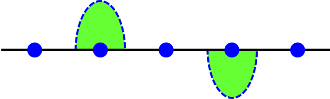
Figure 4.23
\(k_{4} = \frac{2\pi}{a}\) & \(\mathbf{\Gamma}^{(4)}\) & 1 & 1 & 1 & 1 & \(\varphi_{4}\) & 
Figure 4.24 & 
Figure 4.25
()
The basis functions \(\varphi_{\mu}(x)\) must satisfy the following equation:
\[\left( \ 1\ \middle| \ ma\ \right)\varphi_{\mu}(x) = e^{- ik_{\mu}ma}\varphi_{\mu}(x) \nonumber \]
which describes how the symmetry operations (lattice translations) affect the basis function for the IR \(\mathbf{\Gamma}^{(\mu)}\). To illustrate this important feature of basis functions, a real function (yellow half-ellipse with solid red boundary) is placed at the origin lattice point 0. For each IR, the effect of the translation is illustrated: a change of sign flips the half-ellipse with respect to the real line and a change to an imaginary value gives a green half-ellipse with dashed blue boundary.
OBSERVATIONS:
- The characters for the class \(\boldsymbol{T}_{0}\) are all unity, in agreement with the assignment that this translation corresponds to the identity operation of the group.
- Each basis function obeys the periodic boundary condition: \(\varphi_{\mu}(x + 4a) = \varphi_{\mu}(x)\).
- The characters for the IR \(\mathbf{\Gamma}^{(4)}\) are all unity, so this IR is the totally symmetric IR of the lattice group and its basis function \(\varphi_{4}(x)\) has the complete symmetry of the Bravais lattice. The wavevector \(\boldsymbol{k}_{4}\) is \(\frac{2\pi}{a}\), which is a reciprocal lattice vector, so the wavevector \(\boldsymbol{k}_{0} = 0\) also yields the same characters. So, \(\boldsymbol{k}_{0} = 0\) is chosen for the wavevector of this IR rather than \(\boldsymbol{k}_{4} = \frac{2\pi}{a}\).
- The characters for the IR \(\mathbf{\Gamma}^{(2)}\) are the real numbers +1 or –1, so this IR is a real representation of the lattice group. Odd lattice steps change the sign of the basis function; even lattice steps retain the sign of the basis function.
- The IRs \(\mathbf{\Gamma}^{(1)}\) and \(\mathbf{\Gamma}^{(3)}\) have imaginary characters and they occur as complex conjugate pairs. Therefore, their corresponding basis functions are complex conjugates of each other.
The four wavevectors of the four IRs, \(\boldsymbol{k}_{0} = 0,\ \boldsymbol{k}_{1} = \frac{\pi}{2a},\ \boldsymbol{k}_{2} = \frac{\pi}{a},\ \boldsymbol{k}_{3} = \frac{3\pi}{2a},\) represents points in reciprocal space between the two adjacent lattice points \(\boldsymbol{k}_{0} = 0\) and \(\boldsymbol{k}_{4} = \frac{2\pi}{a}\). For this very restricted periodic boundary condition, the allowed wavevectors (“k-points”) form a discrete set that serve as labels for the IRs.
(45) The previous example illustrated how the IRs arise for a set of lattice translations. In the example, the periodic boundary condition was set low, but they are generally selected to be quite large so that \(\boldsymbol{T}_{N_{1}} \equiv \mathbf{0}\) for a large integer \(N_{1}\). The resulting set of \(N_{1}\) wavevectors \(\boldsymbol{k}_{\mu}\) form a set of very closely spaced, quasi-continuous, points in the reciprocal space of the periodic structure. The following summarizes this outcome for 1-d and 3-d Bravais lattices:
1-d Bravais Lattice
\[\mathcal{L =}\left\{ \left( 1 \middle| m\boldsymbol{a}_{1} \right);0 \leq m < N_{1} \right\};\ N_{1}\boldsymbol{a}_{1} \equiv \mathbf{0}. \nonumber \]
- Reciprocal lattice is \(\{\boldsymbol{K}_{h} = h\boldsymbol{a}_{1}^{*}\}\) with \(a_{1}^{*} = \frac{2\pi}{a}\).
- IR representatives are \(\mathbf{\Gamma}^{(\mu)} = e^{- i\boldsymbol{k}_{\mu} \cdot m\boldsymbol{a}}\) with wavevectors \(\boldsymbol{k}_{\mu} = \frac{\mu}{N_{1}}\boldsymbol{a}_{1}^{*}\ (0 \leq \mu < N_{1})\).
- There are \(N_{1}\) classes and N1 IRs.
3-d Bravais Lattice
\[\mathcal{L =}\left\{ \left( 1 \middle| m\boldsymbol{a}_{1} + n\boldsymbol{a}_{2} + p\boldsymbol{a}_{3} \right);0 \leq m < N_{1},\ 0 \leq n < N_{2},0 \leq p < N_{3} \right\}\); \(N_{1}\boldsymbol{a}_{1} \equiv \mathbf{0}\), \({\ N}_{2}\boldsymbol{a}_{2} \equiv \mathbf{0}\), and \({\ N}_{3}\boldsymbol{a}_{3} \equiv \mathbf{0}. \nonumber \]
- Reciprocal lattice is \(\{\boldsymbol{K}_{hkl} = h\boldsymbol{a}_{1}^{*} + k\boldsymbol{a}_{2}^{*} + l\boldsymbol{a}_{3}^{*}\}\).
- IR representatives are \(\mathbf{\Gamma}^{(\mu\nu\omega)} = e^{- i\boldsymbol{k}_{\mu\nu\omega} \cdot \boldsymbol{T}_{mnp}} = \exp\left( - 2\pi i\left( \frac{\mu m}{N_{1}} + \frac{\nu n}{N_{2}} + \frac{\omega p}{N_{3}} \right) \right)\) with wavevectors \(\boldsymbol{k}_{\mu\nu\omega} = \frac{\mu}{N_{1}}\boldsymbol{a}_{1}^{*} + \frac{\nu}{N_{2}}\boldsymbol{a}_{2}^{*} + \frac{\omega}{N_{3}}\boldsymbol{a}_{3}^{*}\ (0 \leq \mu < N_{1};\ 0 \leq \nu < N_{2};\ 0 \leq \omega < N_{3})\).
- There are \(N_{1}N_{2}N_{3}\) classes and \(N_{1}N_{2}N_{3}\) IRs.
Now that we have identified the irreducible representations for the group of lattice translations, what are the basis functions for these IRs? As we pointed out in slide (38), these functions serve as eigenfunctions for the one-electron Schrödinger equation. For the 1-d example, we illustrated important features of these basis functions based upon how they are affected by the various translational symmetry operations of the lattice.