3.3: Significant Figures and Rounding off

Learning Objectives

Make sure you thoroughly understand the following essential ideas which have been presented above. It is especially important that you know the precise meanings of all the highlighted terms in the context of this topic.

• Give an example of a measurement whose number of significant digits is clearly too great, and explain why.
• State the purpose of rounding off, and describe the information that must be known to do it properly.
• Round off a number to a specified number of significant digits.
• Explain how to round off a number whose second-most-significant digit is 9.
• Carry out a simple calculation that involves two or more observed quantities, and express the result in the appropriate number of significant figures.

The numerical values we deal with in science (and in many other aspects of life) represent measurements whose values are never known exactly. Our pocket-calculators or computers don't know this; they treat the numbers we punch into them as "pure" mathematical entities, with the result that the operations of arithmetic frequently yield answers that are physically ridiculous even though mathematically correct. The purpose of this unit is to help you understand why this happens, and show you what to do about it.

Digits: significant and otherwise

• "The population of our city is 157,872."
• "The number of registered voters as of Jan 1 was 27,833."

Consider the two statements shown above. Which of these would you be justified in dismissing immediately? Certainly not the second one, because it probably comes from a database which contains one record for each voter, so the number is found simply by counting the number of records.

The first statement cannot possibly be correct. Even if a city’s population could be defined in a precise way (Permanent residents? Warm bodies?), how can we account for the minute-by minute changes that occur as people are born and die, or move in and move away?

What is the difference between the two population numbers stated above? The first one expresses a quantity that cannot be known exactly– that is, it carries with it a degree of uncertainty. It is quite possible that the last census yielded precisely 157,872 records, and that this might be the “population of the city” for legal purposes, but it is surely not the “true” population. To better reflect this fact, one might list the population (in an atlas, for example) as 157,900 or even 158,000. These two quantities have been rounded off to four and three significant figures, respectively, and the have the following meanings:

• 157900 (the significant digits are underlined here) implies that the population is believed to be within the range of about 157850 to about 157950. In other words, the population is 157900±50. The “plus-or-minus 50” appended to this number means that we consider the absolute uncertainty of the population measurement to be 50 – (–50) = 100. We can also say that the relative uncertainty is 100/157900, which we can also express as 1 part in 1579, or 1/1579 = 0.000633, or about 0.06 percent.
• The value 158000 implies that the population is likely between about 157500 and 158500, or 158000±500. The absolute uncertainty of 1000 translates into a relative uncertainty of 1000/158000 or 1 part in 158, or about 0.6 percent.

Which of these two values we would report as “the population” will depend on the degree of confidence we have in the original census figure; if the census was completed last week, we might round to four significant digits, but if it was a year or so ago, rounding to three places might be a more prudent choice. In a case such as this, there is no really objective way of choosing between the two alternatives.

This illustrates an important point: the concept of significant digits has less to do with mathematics than with our confidence in a measurement. This confidence can often be expressed numerically (for example, the height of a liquid in a measuring tube can be read to ±0.05 cm), but when it cannot, as in our population example, we must depend on our personal experience and judgment.

So, what is a significant digit? According to the usual definition, it is all the numerals in a measured quantity (counting from the left) whose values are considered as known exactly, plus one more whose value could be one more or one less:

• In “157900” (four significant digits), the leftmost three digits are known exactly, but the fourth digit, “9” could well be “8” if the “true value” is within the implied range of 157850 to 157950.
• In “158000” (three significant digits), the leftmost two digits are known exactly, while the third digit could be either “7” or “8” if the true value is within the implied range of 157500 to 158500.

Although rounding off always leads to the loss of numeric information, what we are getting rid of can be considered to be “numeric noise” that does not contribute to the quality of the measurement.

The purpose in rounding off is to avoid expressing a value to a greater degree of precision than is consistent with the uncertainty in the measurement.

Implied Uncertainty and Round-off error

If you know that a balance is accurate to within 0.1 mg, say, then the uncertainty in any measurement of mass carried out on this balance will be ±0.1 mg. Suppose, however, that you are simply told that an object has a length of 0.42 cm, with no indication of its precision. In this case, all you have to go on is the number of digits contained in the data. Thus the quantity “0.42 cm” is specified to 0.01 unit in 0 42, or one part in 42 . The implied relative uncertainty in this figure is 1/42, or about 2%. The precision of any numeric answer calculated from this value is therefore limited to about the same amount.

It is important to understand that the number of significant digits in a value provides only a rough indication of its precision, and that information is lost when rounding off occurs.

Suppose, for example, that we measure the weight of an object as 3.28 g on a balance believed to be accurate to within ±0.05 gram. The resulting value of 3.28±.05 gram tells us that the true weight of the object could be anywhere between 3.23 g and 3.33 g. The absolute uncertainty here is 0.1 g (±0.05 g), and the relative uncertainty is 1 part in 32.8, or about 3 percent.

How many significant digits should there be in the reported measurement? Since only the leftmost “3” in “3.28” is certain, you would probably elect to round the value to 3.3 g. So far, so good. But what is someone else supposed to make of this figure when they see it in your report? The value “3.3 g” suggests an implied uncertainty of 3.3±0.05 g, meaning that the true value is likely between 3.25 g and 3.35 g. This range is 0.02 g below that associated with the original measurement, and so rounding off has introduced a bias of this amount into the result. Since this is less than half of the ±0.05 g uncertainty in the weighing, it is not a very serious matter in itself. However, if several values that were rounded in this way are combined in a calculation, the rounding-off errors could become significant.

The standard rules for rounding off are well known. Before we set them out, let us agree on what to call the various components of a numeric value.

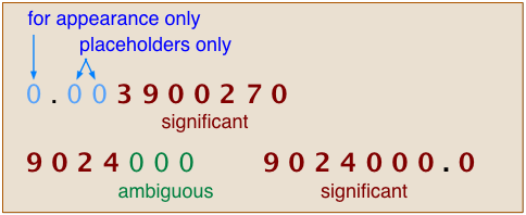
• The most significant digit is the leftmost digit (not counting any leading zeros which function only as placeholders and are never significant digits.)
• If you are rounding off to n significant digits, then the least significant digit is the nth digit from the most significant digit.The least significant digit can be a zero.
• The first non-significant digit is the n+1th digit.

• If the first non-significant digit is less than 5, then the least significant digit remains unchanged.
• If the first non-significant digit is greater than 5, the least significant digit is incremented by 1.
• If the first non-significant digit is 5, the least significant digit can either be incremented or left unchanged (see below!)
• All non-significant digits are removed.

Students are sometimes told to increment the least significant digit by 1 if it is odd, and to leave it unchanged if it is even. One wonders if this reflects some idea that even numbers are somehow “better” than odd ones! (The ancient superstition is just the opposite, that only the odd numbers are "lucky".)

In fact, you could do it equally the other way around, incrementing only the even numbers. If you are only rounding a single number, it doesn’t really matter what you do. However, when you are rounding a series of numbers that will be used in a calculation, if you treated each first-nonsignificant 5 in the same way, you would be over- or underestimating the value of the rounded number, thus accumulating round-off error. Since there are equal numbers of even and odd digits, incrementing only the one kind will keep this kind of error from building up.

You could do just as well, of course, by flipping a coin!

Table: Examples of rounding-off

number to round / no. of sig. digits	result	comment
34.216 / 3	34.2	First non-significant digit (1) is less than 5, so number is simply truncated.
2.252 / 2	2.2 or 2.3	First non-significant digit is 5, so least sig. digit can either remain unchanged or be incremented.
39.99 / 3	40.0	Crossing "decimal boundary", so all numbers change.
85,381 / 3	85,400	The two zeros are just placeholders
0.04597 / 3	0.0460	The two leading zeros are not significant digits.

Rounding Up The Nines

Suppose that an object is found to have a weight of 3.98 ± 0.05 g. This would place its true weight somewhere in the range of 3.93 g to 4.03 g. In judging how to round this number, you count the number of digits in “3.98” that are known exactly, and you find none! Since the “4” is the leftmost digit whose value is uncertain, this would imply that the result should be rounded to one significant figure and reported simply as 4 g. An alternative would be to bend the rule and round off to two significant digits, yielding 4.0 g. How can you decide what to do?

In a case such as this, you should look at the implied uncertainties in the two values, and compare them with the uncertainty associated with the original measurement.

rounded value	implied max	implied min	absolute uncertainty	relative uncertainty
3.98 g	3.985 g	3.975 g	±.005 g or 0.01 g	1 in 400, or 0.25%
4 g	4.5 g	3.5 g	±.5 g or 1 g	1 in 4, 25%
4.0 g	4.05 g	3.95 g	±.05 g or 0.1 g	1 in 40, 2.5%

Clearly, rounding off to two digits is the only reasonable course in this example.

The same kind of thing could happen if the original measurement was 9.98 ± 0.05 g. Again, the true value is believed to be in the range of 10.03 g to 9.93 g. The fact that no digit is certain here is an artifact of decimal notation. The absolute uncertainty in the observed value is 0.1 g, so the value itself is known to about 1 part in 100, or 1%. Rounding this value to three digits yields 10.0 g with an implied uncertainty of ±.05 g, or 1 part in 100, consistent with the uncertainty in the observed value.

Observed values should be rounded off to the number of digits that most accurately conveys the uncertainty in the measurement.

• Usually, this means rounding off to the number of significant digits in in the quantity; that is, the number of digits (counting from the left) that are known exactly, plus one more.
• When this cannot be applied (as in the example above when addition of subtraction of the absolute uncertainty bridges a power of ten), then we round in such a way that the relative implied uncertainty in the result is as close as possible to that of the observed value.

Rounding off the Results of Calculations

When carrying out calculations that involve multiple steps, you should avoid doing any rounding until you obtain the final result. In science, we frequently need to carry out calculations on measured values. For example, you might use your pocket calculator to work out the area of a rectangle:

Your calculator is of course correct as far as the pure numbers go, but you would be wrong to write down 1.57676 cm² as the answer. Two possible options for rounding off the calculator answer are shown below:

Rounded Value	Precision
1.58	1 part in 158, or 0.6%
1.6	1 part in 16, or 6 %

It is clear that neither option is entirely satisfactory; rounding to 3 significant digits leaves the answer too precisely specified, whereas following the rule and rounding to 2 digits has the effect of throwing away some precision. In this case, it could be argued that rounding to three digits is justified because the implied relative uncertainty in the answer, 0.6%, is more consistent with those of the two factors.

The above example is intended to point out that the rounding-off rules, although convenient to apply, do not always yield the most desirable result. When in doubt, it is better to rely on relative implied uncertainties.

Addition and Subtraction

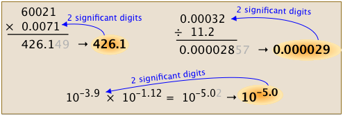
When adding or subtracting, we go by the number of decimal places rather than by the number of significant digits. Identify the quantity having the smallest number of decimal places, and use this number to set the number of decimal places in the answer.

Multiplication and Division

The result must contain the same number of significant figures as in the value having the least number of significant figures.

Logarithms and Antilogarithms

Express the base-10 logarithm of a value using the same number of significant figures as is present in the normalized form of that value. Similarly, for antilogarithms (numbers expressed as powers of 10), use the same number of significant figures as are in that power.

mean?

If a number is expressed in the form a × 10^b ("scientific notation") with the additional restriction that the coefficient a is no less than 1 and less than 10, the number is in its normalized form.

More Rounding Examples

The following examples will illustrate the most common problems you are likely to encounter in rounding off the results of calculations. They deserve your careful study!

calculator result	rounded	remarks
	1.6	Rounding to two significant figures yields an implied uncertainty of 1/16 or 6%, three times greater than that in the least-preciseely known factor. This is a good illustration of how rounding can lead to the loss of information.
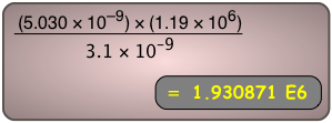
	1.9E6	The "3.1" factor is specified to 1 part in 31, or 3%. In the answer 1.9, the value is expressed to 1 part in 19, or 5%. These precisions are comparable, so the rounding-off rule has given us a reasonable result.
A certain book has a thickness of 117 mm; find the height of a stack of 24 identical books:	2810 mm	The “24” and the “1” are exact, so the only uncertain value is the thickness of each book, given to 3 significant digits. The trailing zero in the answer is only a placeholder.
	10.4	In addition or subtraction, look for the term having the smallest number of decimal places, and round off the answer to the same number of places.
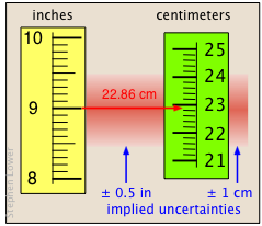
	23 cm	[see below]

The last of the examples shown above represents the very common operation of converting one unit into another. There is a certain amount of ambiguity here; if we take "9 in" to mean a distance in the range 8.5 to 9.5 in, then the uncertainty is ±0.5 in, which is 1 part in 18, or about ± 6%. The relative uncertainty in the answer must be the same, since all the values are multiplied by the same factor, 2.54 cm/in. In this case we are justified in writing the answer to two significant digits, yielding an uncertainty of about ±4 cm; if we had used the answer "20 cm" (one significant digit), its implied uncertainty would be ±5 cm, or ±25%.

When the appropriate number of significant digits is in question, calculating the relative uncertainty can help you decide.