3.2: The Meaning of Measure

Learning Objectives

Make sure you thoroughly understand the following essential ideas which have been presented above. It is especially important that you know the precise meanings of all the highlighted terms in the context of this topic.

• Give an example of a measured numerical value, and explain what distinguishes it from a "pure" number.
• Give examples of random and systematic errors in measurements.
• Find the mean value of a series of similar measurements.
• State the principal factors that affect the difference between the mean value of a series of measurements, and the "true value" of the quantity being measured.
• Calculate the absolute and relative precisions of a given measurement, and explain why the latter is generally more useful.
• Distinguish between the accuracy and the precision of a measured value, and on the roles of random and systematic error.

The exact distance between the upper lip and the tip of the dorsal fin will forever be hidden in a fog of uncertainty. The angle at which we hold the calipers and the force with which we close them on the object will never be exactly reproducible. A more fundamental limitation occurs whenever we try to compare a continuously-varying quantity such as distance with the fixed intervals on a measuring scale; between 59 and 60 mils there is the same infinity of distances that exists between 59 and 60 miles!

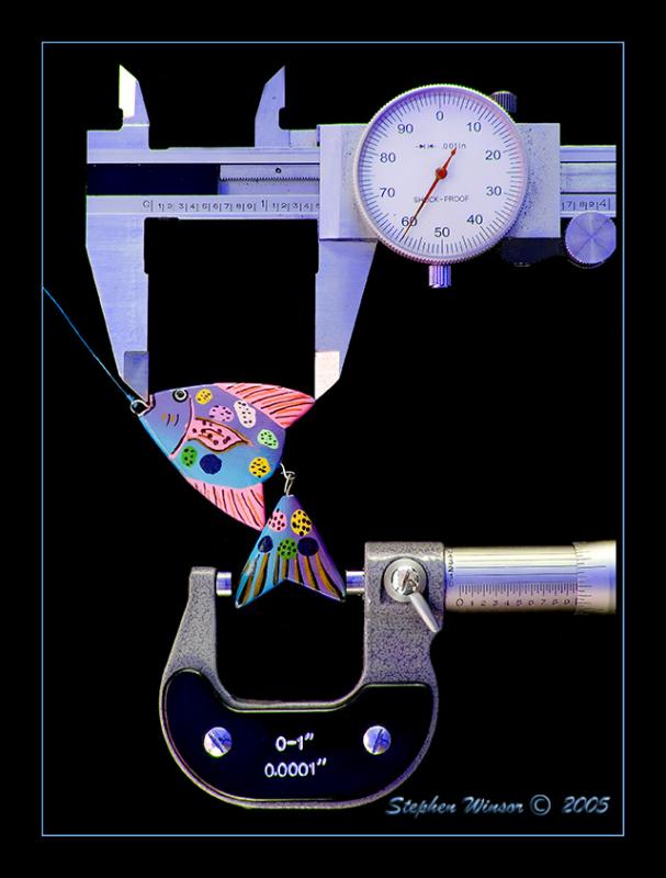
Image by Stephen Winsor; used with permission of the artist.

The "true value" of a measured quantity, if it exists at all, will always elude us; the best we can do is learn how to make meaningful use (and to avoid mis-use!) of the numbers we read off of our measuring devices.

Uncertainty is Certain!

In science, there are numbers and there are "numbers". What we ordinarily think of as a "number" and will refer to here as a pure number is just that: an expression of a precise value. The first of these you ever learned were the counting numbers, or integers; later on, you were introduced to the decimal numbers, and the rational numbers, which include numbers such as 1/3 and π (pi) that cannot be expressed as exact decimal values.

The other kind of numeric quantity that we encounter in the natural sciences is a measured value of something– the length or weight of an object, the volume of a fluid, or perhaps the reading on an instrument. Although we express these values numerically, it would be a mistake to regard them as the kind of pure numbers described above.

Confusing? Suppose our instrument has an indicator such as you see here. The pointer moves up and down so as to display the measured value on this scale. What number would you write in your notebook when recording this measurement? Clearly, the value is somewhere between 130 and 140 on the scale, but the graduations enable us to be more exact and place the value between 134 and 135. The indicator points more closely to the latter value, and we can go one more step by estimating the value as perhaps 134.8, so this is the value you would report for this measurement.

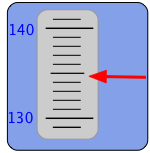
Now here’s the important thing to understand: although “134.8” is itself a number, the quantity we are measuring is almost certainly not 134.8— at least, not exactly. The reason is obvious if you note that the instrument scale is such that we are barely able to distinguish between 134.7, 134.8, and 134.9. In reporting the value 134.8 we are effectively saying that the value is probably somewhere with the range 134.75 to 134.85. In other words, there is an uncertainty of ±0.05 unit in our measurement.

All measurements of quantities that can assume a continuous range of values (lengths, masses, volumes, etc.) consist of two parts: the reported value itself (never an exactly known number), and the uncertainty associated with the measurement. By “error”, we do not mean just outright mistakes, such as incorrect use of an instrument or failure to read a scale properly; although such gross errors do sometimes happen, they usually yield results that are sufficiently unexpected to call attention to themselves.

Errors in Measurements

All measurements are subject to error which contributes to the uncertainty of the result. By “error”, we do not mean just outright mistakes, such as incorrect use of an instrument or failure to read a scale properly; although such gross errors do sometimes happen, they usually yield results that are sufficiently unexpected to call attention to themselves.

When you measure a volume or weight, you observe a reading on a scale of some kind. Scales, by their very nature, are limited to fixed increments of value, indicated by the division marks. The actual quantities we are measuring, in contrast, can vary continuously, so there is an inherent limitation in how finely we can discriminate between two values that fall between the marked divisions of the measuring scale. The same problem remains if we substitute an instrument with a digital display; there will always be some point at which some value that lies between the two smallest divisions must arbitrarily toggle between two numbers on the readout display. This introduces an element of randomness into the value we observe, even if the "true" value remains unchanged.

The more sensitive the measuring instrument, the less likely it is that two successive measurements of the same sample will yield identical results. In the example we discussed above, distinguishing between the values 134.8 and 134.9 may be too difficult to do in a consistent way, so two independent observers may record different values even when viewing the same reading. Each measurement is also influenced by a myriad of minor events, such as building vibrations, electrical fluctuations, motions of the air, and friction in any moving parts of the instrument. These tiny influences constitute a kind of "noise" that also has a random character. Whether we are conscious of it or not, all measured values contain an element of random error.

Each measurement is also influenced by a myriad of minor events, such as building vibrations, electrical fluctuations, motions of the air, and friction in any moving parts of the instrument. These tiny influences constitute a kind of "noise" that also has a random character. Whether we are conscious of it or not, all measured values contain an element of random error.

Suppose that you weigh yourself on a bathroom scale, not noticing that the dial reads “1.5 kg” even before you have placed your weight on it. Similarly, you might use an old ruler with a worn-down end to measure the length of a piece of wood. In both of these examples, all subsequent measurements, either of the same object or of different ones, will be off by a constant amount. Unlike random error, which is impossible to eliminate, these systematic errors are usually quite easy to avoid or compensate for, but only by a conscious effort in the conduct of the observation, usually by proper zeroing and calibration of the measuring instrument. However, once systematic error has found its way into the data, it is can be very hard to detect.

The Difference Between Accuracy and Precision

We tend to use these two terms interchangeably in our ordinary conversation, but in the context of scientific measurement, they have very different meanings:

• Accuracy refers to how closely the measured value of a quantity corresponds to its “true” value.
• Precision expresses the degree of reproducibility, or agreement between repeated measurements.

Accuracy, of course, is the goal we strive for in scientific measurements. Unfortunately, however, there is no obvious way of knowing how closely we have achieved it; the “true” value, whether it be of a well-defined quantity such as the mass of a particular object, or an average that pertains to a collection of objects, can never be known– and thus we can never recognize it if we are fortunate enough to find it.

A target on a dart board serves as a convenient analogy. The results of four sets of measurements (or four dart games) are illustrated below. Each set is made up of ten observations (or throws of darts.) Each red dot corresponds to the point at which a dart has hit the target — or alternatively, to the value of an individual observation. For measurements, assume the true value of the quantity being measured lies at the center of each target.

Now consider the following four sets of results:

- Right on! You win the dart game, and get an A grade on your measurement results.

- Your results are beautifully replicable, but your measuring device may not have been calibrated properly or your observations suffer from a systematic error of some kind. Accuracy: F, Precision, A; overall grade C.

- Extremely unlikely, and probably due to pure luck; the only reason for the accurate mean is that your misses mostly canceled out. Grade D.

- Pretty sad; consider switching to music or politics — or have your eyes examined.

Note carefully that when we make real measurements, there is no dart board or target that enables one to immediately judge the quality of the result. If we make only a few observations, we may be unable distinguish between any of these scenarios. Thus we cannot distinguish between the four scenarios illustrated above by simply examining the results of the two measurements. We can, however, judge the precision of the results, and then apply simple statistics to estimate how closely the mean value is likely to reflect the true value in the absence of systematic error.

More than one answer in Replicate Measurements

If you wish to measure your height to the nearest centimeter or inch, or the volume of a liquid cooking ingredient to the nearest “cup”, you can probably do so without having to worry about random error. The error will still be present, but its magnitude will be such a small fraction of the value that it will not be detected. Thus random error is not something we worry about too much in our daily lives.

If we are making scientific observations, however, we need to be more careful, particularly if we are trying to exploit the full sensitivity of our measuring instruments in order to achieve a result that is as reliable as possible. If we are measuring a directly observable quantity such as the weight or volume of an object, then a single measurement, carefully done and reported to a precision that is consistent with that of the measuring instrument, will usually be sufficient.

More commonly, however, we are called upon to find the value of some quantity whose determination depends on several other measured values, each of which is subject to its own sources of error. Consider a common laboratory experiment in which you must determine the percentage of acid in a sample of vinegar by observing the volume of sodium hydroxide solution required to neutralize a given volume of the vinegar. You carry out the experiment and obtain a value. Just to be on the safe side, you repeat the procedure on another identical sample from the same bottle of vinegar. If you have actually done this in the laboratory, you will know it is highly unlikely that the second trial will yield the same result as the first. In fact, if you run a number of replicate (that is, identical in every way) determinations, you will probably obtain a scatter of results.

To understand why, consider all the individual measurements that go into each determination; the volume of the vinegar sample, your judgment of the point at which the vinegar is neutralized, and the volume of solution used to reach this point. And how accurately do you know the concentration of the sodium hydroxide solution, which was made up by dissolving a measured weight of the solid in water and then adding more water until the solution reaches some measured volume. Each of these many observations is subject to random error; because such errors are random, they can occasionally cancel out, but for most trials we will not be so lucky– hence the scatter in the results.

A similar difficulty arises when we need to determine some quantity that describes a collection of objects. For example, a pharmaceutical researcher will need to determine the time required for half of a standard dose of a certain drug to be eliminated by the body, or a manufacturer of light bulbs might want to know how many hours a certain type of light bulb will operate before it burns out. In these cases a value for any individual sample can be determined easily enough, but since no two samples (patients or light bulbs) are identical, we are compelled to repeat the same measurement on multiple samples, and once again, are faced with a scattering of results.

As a final example, suppose that you wish to determine the diameter of a certain type of coin. You make one measurement and record the results. If you then make a similar measurement along a different cross-section of the coin, you will likely get a different result. The same thing will happen if you make successive measurements on other coins of the same kind.

Here we are faced with two kinds of problems. First, there is the inherent limitation of the measuring device: we can never reliably measure more finely than the marked divisions on the ruler. Secondly, we cannot assume that the coin is perfectly circular; careful inspection will likely reveal some distortion resulting from a slight imperfection in the manufacturing process. In these cases, it turns out that there is no single, true value of either quantity we are trying to measure.

Mean, Median, and Range of a Series of Observations

There are a variety of ways to express the average, or central tendency of a series of measurements, with mean (more precisely, arithmetic mean) being most commonly employed. Our ordinary use of the term "average" also refers to the mean. When we obtain more than one result for a given measurement (either made repeatedly on a single sample, or more commonly, on different samples), the simplest procedure is to report the mean, or average value. The mean is defined mathematically as the sum of the values, divided by the number of measurements:

\[x_m = \dfrac{\displaystyle \sum_i x_i}{n} \label{mean}\]

If you are not familiar with this notation, don’t let it scare you! Take a moment to see how it expresses the previous sentence; if there are \(n\) measurements, each yielding a value xI, then we sum over all \(i\) and divide by \(n\) to get the mean value \(x_m\). For example, if there are only two measurements, \(x_1\) and \(x_1\), then the mean is \((x_1 + x_2)/2\).

Example \(\PageIndex{1}\)

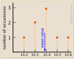
Calculate the mean value of the set of eight measurements illustrated here.

Solution

There are eight data points (10.4 was found in three trials, 10.5 in two), so \(n=8\). The mean is (via Equation \ref{mean}):

\[ \dfrac{10.2+10.3+(3 x 10.4) + 10.5+10.5+10.8}{8} = 10.4. \nonumber\]

Range

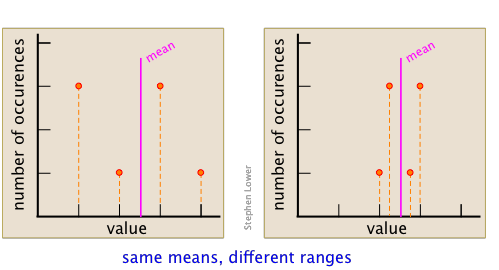
The range of a data set is the difference between its smallest and largest values. As such, its value reflects the precision of the result. For example, the following data sets have the same average, but the one having the smaller range is clearly more precise.

If you arrange the list of measured values in order of their magnitude, the median is the one that has as many values above it as below it.

Examples: for the data set [22 23 23 24 26 28] the mode would be 23.

For an odd number of values n, the median is the [(n+1)/2]th member of the set. Thus for [22 23 23 24 24 27], (n+1)/2 =3, so 23 is the median value.

Mode

This refers to the value that is observed most frequently in a series of measurements. If two or more values tie for the highest frequency, then there can be multiple modes. Mode is most useful in describing larger data sets.

Example: for the data set [22 23 23 24 26 26] the modes are 23 and 24.

The more observations, the more reliable the mean value. If this is not immediately obvious, think about it this way. You would not want to predict the outcome of the next election on the basis of interviews with only two or three voters; you would want a sample of ten to twenty at a minimum, and if the election is an important national one, a fair sample would require hundreds to thousands of people distributed over the entire geographic area and representing a variety of socio-economic groups. Similarly, you would want to test a large number of light bulbs in order to estimate the mean lifetime of bulbs of that type.

Statistical theory tells us that the more samples we have, the greater will be the chance that the mean of the results will correspond to the “true” value, which in this case would be the mean obtained if samples could be taken from the entire population (of people or of light bulbs.)

This point can be better appreciated by examining the two sets of data shown here. The set on the left consists of only three points (shown in orange), and gives a mean that is quite far removed from the "true" value, which is arbitrarily chosen for this example.

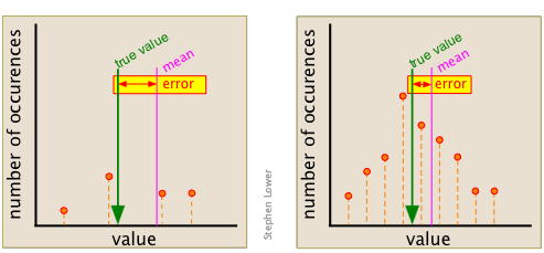
In the data set on the right, composed of nine measurements, the deviation of the mean from the true value is much smaller.

Deviation of the mean from the "true value" becomes smaller when more measurements are made.

Plots and points

A similar problem arises when you try to fit a curve to a series of plotted points. Suppose, for example, that curve 1 (red) represents the true relationship between the quantities indicated on the y-axis (dependent variable) and those on the x-axis (independent variable). This curve is derived from the seven points indicated on the plot.

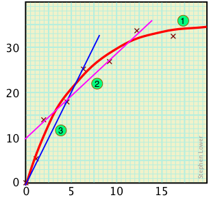
Contrast this curve with the false straight-line relationships that might be obtained if only four or three points had been recorded.

Absolute and Relative Uncertainty

If you weigh out 74.1 mg of a solid sample on a laboratory balance that is accurate to within 0.1 milligram, then the actual weight of the sample is likely to fall somewhere in the range of 74.0 to 74.2 mg; the absolute uncertainty in the weight you observe is 0.2 mg, or ±0.1 mg. If you use the same balance to weigh out 3.2914 g of another sample, the actual weight is between 3.2913 g and 3.2915 g, and the absolute uncertainty is still ±0.1 mg. Thus the absolute uncertainty is is unrelated to the magnitude of the observed value.

When expressing the uncertainty of a value given in scientific notation, the exponential part should include both the value itself and the uncertainty. An example of the proper form would be (3.19 ± 0.02) × 10⁴ m.

Although the absolute uncertainties in these two examples are identical, we would probably consider the second measurement to be more precise because the uncertainty is a smaller fraction of the measured value. A quantity calculated in this way is known as the relative uncertainty.

Example \(\PageIndex{1}\)

Calculate the relative uncertainties of the following absolute uncertainties:

1. 74.1 ± 0.1 mg,
2. 3.2914 ± 0.1 mg.

Solution

1. \[\dfrac{0.2\, mg}{74.1\, mg} = 0.0027\, \text{or} \, 0.003 \nonumber\] (note that the quotient is dimensionless) this can be expressed as 0.3% (3 parts per hundred) or 3 parts per thousand.
2. \[\dfrac{0.0002 \,g}{3.2913\, g} = 8.4 \times 10^{-5} \, \text{or roughly} \,8 \times 10^{-5} \nonumber\], which we can express as \(8 \times 10^{-3}\%\) (0.008 parts per hundred), or (8E–5 / 10) = 8E–6 = 8 PPM.

Relative uncertainties are widely used to express the reliability of measurements, even those for a single observation, in which case the uncertainty is that of the measuring device. Relative uncertainties can be expressed as parts per hundred (percent), per thousand (PPT), per million, (PPM), and so on.

Propagation of Error

We are often called upon to find the value of some quantity whose determination depends on several other measured values, each of which is subject to its own sources of error.

Consider a common laboratory experiment in which you must determine the percentage of acid in a sample of vinegar by observing the volume of sodium hydroxide solution required to neutralize a given volume of the vinegar. You carry out the experiment and obtain a value. Just to be on the safe side, you repeat the procedure on another identical sample from the same bottle of vinegar. If you have actually done this in the laboratory, you will know it is highly unlikely that the second trial will yield the same result as the first. In fact, if you run a number of replicate (that is, identical in every way) determinations, you will probably obtain a scatter of results.

To understand why, consider all the individual measurements that go into each determination; the volume of the vinegar sample, your judgement of the point at which the vinegar is neutralized, and the volume of solution used to reach this point. And how accurately do you know the concentration of the sodium hydroxide solution, which was made up by dissolving a measured weight of the solid in water and then adding more water until the solution reaches some measured volume. Each of these many observations is subject to random error; because such errors are random, they can occasionally cancel out, but for most trials we will not be so lucky — hence the scatter in the results.

Rules for estimating errors in calculated results

Suppose you measure the mass and volume of a sample, and are required to calculate its density by dividing one quantity by the other:

\[d = m / V. \nonumber\]

Both components of this quotient have uncertainties associated with them, and you wish to attach an uncertainty to the calculated density. The general problem of determining the uncertainty of a calculated result turns out to be rather more complicated than you might think, and will not be treated here. There are, however, some very simple rules that are sufficient for most practical purposes.

• Addition and subtraction, both numbers have uncertainties: The simplest method is to just add the absolute uncertainties.
• Multiplication or division, both numbers have uncertainties: Convert the absolute uncertainties into relative uncertainties, and add these. Or better, add their squares and take the square root of the sum.
• Multiplication or division by a pure number: Trivial case; multiply or divide the uncertainty by the pure number.

Example \(\PageIndex{2}\): Addition and Subtraction of Numbers with Uncertainties

\[(6.3 ± 0.05 \,cm) – (2.1 ± 0.05 \,cm) = 4.2 ± 0.10\,cm \nonumber\]

However, this tends to over-estimate the uncertainty by assuming the worst possible case in which the error in one of the quantities is at its maximum positive value, while that of the other quantity is at its maximum minimum value.

Statistical theory informs us that a more realistic value for the uncertainty of a sum or difference is to add the squares of each absolute uncertainty, and then take the square root of this sum. Applying this to the above values, we have

\[\sqrt{(0.05)^2 + (0.05)^2} = 0.07 \nonumber\]

so the result is 4.2 ± 0.07 cm.

Example \(\PageIndex{3}\)

Estimate the absolute error in the density calculated by dividing (12.7 ± 0.05\, g) by (10.0 ± 0.02\, mL).

Solution

Relative uncertainty of the mass:

\[\dfrac{0.05}{12.7} = 0.0039 = 0.39\% \nonumber\]

Relative uncertainty of the volume:

\[\dfrac{0.02}{10.0} = 0.002 = 0.2\% \nonumber\]

Relative uncertainty of the density:

\[ \sqrt{ (0.39)^2 + (0.2)^2} = 0.44 \% \nonumber\]

Mass ÷ volume:

\[(12.7\, g) ÷ (10.0 \,mL) = 1.27 \,g \,mL^{–1} \nonumber \]

Absolute uncertainty of the density:

\[(± 0.044) \times (1.27 \,g \,mL^{–1}) = ±0.06\, g\, mL^{–1} \nonumber \]