
12: Solubility Equilibria
- Page ID
- 3572

\( \newcommand{\vecs}[1]{\overset { \scriptstyle \rightharpoonup} {\mathbf{#1}} } \)
\( \newcommand{\vecd}[1]{\overset{-\!-\!\rightharpoonup}{\vphantom{a}\smash {#1}}} \)
\( \newcommand{\dsum}{\displaystyle\sum\limits} \)
\( \newcommand{\dint}{\displaystyle\int\limits} \)
\( \newcommand{\dlim}{\displaystyle\lim\limits} \)
\( \newcommand{\id}{\mathrm{id}}\) \( \newcommand{\Span}{\mathrm{span}}\)
( \newcommand{\kernel}{\mathrm{null}\,}\) \( \newcommand{\range}{\mathrm{range}\,}\)
\( \newcommand{\RealPart}{\mathrm{Re}}\) \( \newcommand{\ImaginaryPart}{\mathrm{Im}}\)
\( \newcommand{\Argument}{\mathrm{Arg}}\) \( \newcommand{\norm}[1]{\| #1 \|}\)
\( \newcommand{\inner}[2]{\langle #1, #2 \rangle}\)
\( \newcommand{\Span}{\mathrm{span}}\)
\( \newcommand{\id}{\mathrm{id}}\)
\( \newcommand{\Span}{\mathrm{span}}\)
\( \newcommand{\kernel}{\mathrm{null}\,}\)
\( \newcommand{\range}{\mathrm{range}\,}\)
\( \newcommand{\RealPart}{\mathrm{Re}}\)
\( \newcommand{\ImaginaryPart}{\mathrm{Im}}\)
\( \newcommand{\Argument}{\mathrm{Arg}}\)
\( \newcommand{\norm}[1]{\| #1 \|}\)
\( \newcommand{\inner}[2]{\langle #1, #2 \rangle}\)
\( \newcommand{\Span}{\mathrm{span}}\) \( \newcommand{\AA}{\unicode[.8,0]{x212B}}\)
\( \newcommand{\vectorA}[1]{\vec{#1}} % arrow\)
\( \newcommand{\vectorAt}[1]{\vec{\text{#1}}} % arrow\)
\( \newcommand{\vectorB}[1]{\overset { \scriptstyle \rightharpoonup} {\mathbf{#1}} } \)
\( \newcommand{\vectorC}[1]{\textbf{#1}} \)
\( \newcommand{\vectorD}[1]{\overrightarrow{#1}} \)
\( \newcommand{\vectorDt}[1]{\overrightarrow{\text{#1}}} \)
\( \newcommand{\vectE}[1]{\overset{-\!-\!\rightharpoonup}{\vphantom{a}\smash{\mathbf {#1}}}} \)
\( \newcommand{\vecs}[1]{\overset { \scriptstyle \rightharpoonup} {\mathbf{#1}} } \)
\(\newcommand{\longvect}{\overrightarrow}\)
\( \newcommand{\vecd}[1]{\overset{-\!-\!\rightharpoonup}{\vphantom{a}\smash {#1}}} \)
\(\newcommand{\avec}{\mathbf a}\) \(\newcommand{\bvec}{\mathbf b}\) \(\newcommand{\cvec}{\mathbf c}\) \(\newcommand{\dvec}{\mathbf d}\) \(\newcommand{\dtil}{\widetilde{\mathbf d}}\) \(\newcommand{\evec}{\mathbf e}\) \(\newcommand{\fvec}{\mathbf f}\) \(\newcommand{\nvec}{\mathbf n}\) \(\newcommand{\pvec}{\mathbf p}\) \(\newcommand{\qvec}{\mathbf q}\) \(\newcommand{\svec}{\mathbf s}\) \(\newcommand{\tvec}{\mathbf t}\) \(\newcommand{\uvec}{\mathbf u}\) \(\newcommand{\vvec}{\mathbf v}\) \(\newcommand{\wvec}{\mathbf w}\) \(\newcommand{\xvec}{\mathbf x}\) \(\newcommand{\yvec}{\mathbf y}\) \(\newcommand{\zvec}{\mathbf z}\) \(\newcommand{\rvec}{\mathbf r}\) \(\newcommand{\mvec}{\mathbf m}\) \(\newcommand{\zerovec}{\mathbf 0}\) \(\newcommand{\onevec}{\mathbf 1}\) \(\newcommand{\real}{\mathbb R}\) \(\newcommand{\twovec}[2]{\left[\begin{array}{r}#1 \\ #2 \end{array}\right]}\) \(\newcommand{\ctwovec}[2]{\left[\begin{array}{c}#1 \\ #2 \end{array}\right]}\) \(\newcommand{\threevec}[3]{\left[\begin{array}{r}#1 \\ #2 \\ #3 \end{array}\right]}\) \(\newcommand{\cthreevec}[3]{\left[\begin{array}{c}#1 \\ #2 \\ #3 \end{array}\right]}\) \(\newcommand{\fourvec}[4]{\left[\begin{array}{r}#1 \\ #2 \\ #3 \\ #4 \end{array}\right]}\) \(\newcommand{\cfourvec}[4]{\left[\begin{array}{c}#1 \\ #2 \\ #3 \\ #4 \end{array}\right]}\) \(\newcommand{\fivevec}[5]{\left[\begin{array}{r}#1 \\ #2 \\ #3 \\ #4 \\ #5 \\ \end{array}\right]}\) \(\newcommand{\cfivevec}[5]{\left[\begin{array}{c}#1 \\ #2 \\ #3 \\ #4 \\ #5 \\ \end{array}\right]}\) \(\newcommand{\mattwo}[4]{\left[\begin{array}{rr}#1 \amp #2 \\ #3 \amp #4 \\ \end{array}\right]}\) \(\newcommand{\laspan}[1]{\text{Span}\{#1\}}\) \(\newcommand{\bcal}{\cal B}\) \(\newcommand{\ccal}{\cal C}\) \(\newcommand{\scal}{\cal S}\) \(\newcommand{\wcal}{\cal W}\) \(\newcommand{\ecal}{\cal E}\) \(\newcommand{\coords}[2]{\left\{#1\right\}_{#2}}\) \(\newcommand{\gray}[1]{\color{gray}{#1}}\) \(\newcommand{\lgray}[1]{\color{lightgray}{#1}}\) \(\newcommand{\rank}{\operatorname{rank}}\) \(\newcommand{\row}{\text{Row}}\) \(\newcommand{\col}{\text{Col}}\) \(\renewcommand{\row}{\text{Row}}\) \(\newcommand{\nul}{\text{Nul}}\) \(\newcommand{\var}{\text{Var}}\) \(\newcommand{\corr}{\text{corr}}\) \(\newcommand{\len}[1]{\left|#1\right|}\) \(\newcommand{\bbar}{\overline{\bvec}}\) \(\newcommand{\bhat}{\widehat{\bvec}}\) \(\newcommand{\bperp}{\bvec^\perp}\) \(\newcommand{\xhat}{\widehat{\xvec}}\) \(\newcommand{\vhat}{\widehat{\vvec}}\) \(\newcommand{\uhat}{\widehat{\uvec}}\) \(\newcommand{\what}{\widehat{\wvec}}\) \(\newcommand{\Sighat}{\widehat{\Sigma}}\) \(\newcommand{\lt}{<}\) \(\newcommand{\gt}{>}\) \(\newcommand{\amp}{&}\) \(\definecolor{fillinmathshade}{gray}{0.9}\)Make sure you thoroughly understand the following essential ideas:
- Discuss the roles of lattice- and hydration energy in determining the solubility of a salt in water.
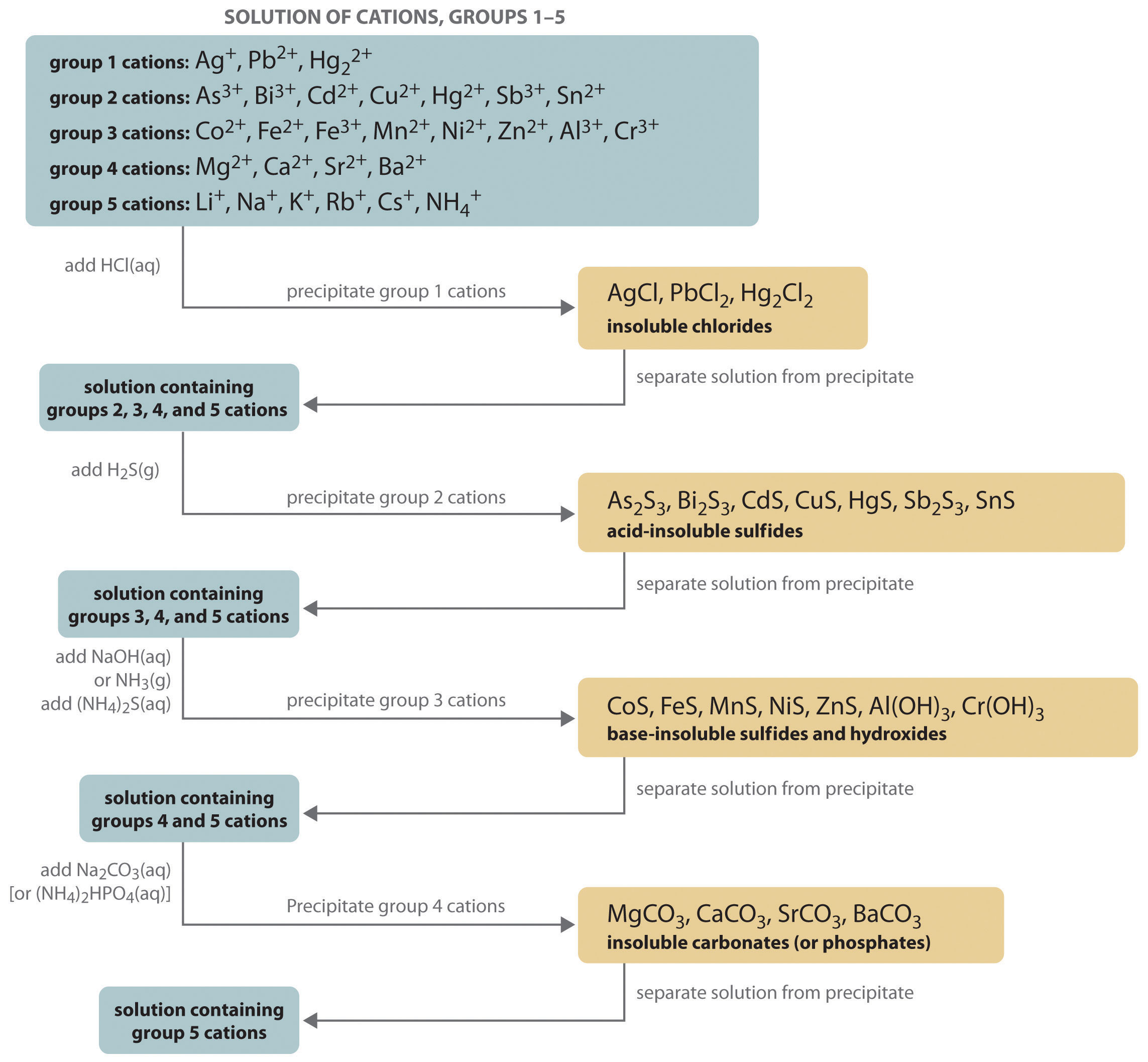
- Explain what a qualitative analysis separation scheme is, and how it works.
- Write the solubility product expression for a salt, given its formula.
- Explain the distinction between an ion product and a solubility product.
- Given the formula of a salt and its Ks value, calculate the molar solubility.
- Explain the Le Chatelier principle leads to the common ion effect.
- Explain why a strong acid such as HCl will dissolve a sparingly soluble salt of a weak acid, but not a salt of a strong acid.
- Describe what happens (and why) when aqueous ammonia is slowly added to a solution of silver nitrate
Dissolution of a salt in water is a chemical process that is governed by the same laws of chemical equilibrium that apply to any other reaction. There are, however, a number of special aspects of of these equilibria that set them somewhat apart from the more general ones that are covered in the lesson set devoted specifically to chemical equilibrium. These include such topics as the common ion effect, the influence of pH on solubility, supersaturation, and some special characteristics of particularly important solubility systems.
Solubility: the dissolution of salts in water
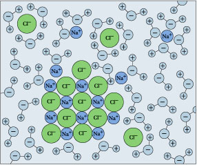
Drop some ordinary table salt into a glass of water, and watch it "disappear". We refer to this as dissolution, and we explain it as a process in which the sodium and chlorine units break away from the crystal surface, get surrounded by H2O molecules, and become hydrated ions.
\[NaCl_{(s)} \rightarrow Na^+_{(aq)}+ Cl^–_{(aq)} \]
The designation (aq) means "aqueous" and comes from aqua, the Latin word for water. It is used whenever we want to emphasize that the ions are hydrated — that H2O molecules are attached to them.
Remember that solubility equilibrium and the calculations that relate to it are only meaningful when both sides (solids and dissolved ions) are simultaneously present. But if you keep adding salt, there will come a point at which it no longer seems to dissolve. If this condition persists, we say that the salt has reached its solubility limit, and the solution is saturated in NaCl. The situation is now described by
\[NaCl_{(s)} \rightleftharpoons Na^+_{(aq)}+ Cl^–_{(aq)}\]
in which the solid and its ions are in equilibrium.
Salt solutions that have reached or exceeded their solubility limits (usually 36-39 g per 100 mL of water) are responsible for prominent features of the earth's geochemistry. They typically form when NaCl leaches from soils into waters that flow into salt lakes in arid regions that have no natural outlets; subsequent evaporation of these brines force the above equilibrium to the left, forming natural salt deposits. These are often admixed with other salts, but in some cases are almost pure NaCl. Many parts of the world contain buried deposits of NaCl (known as halite) that formed from the evaporation of ancient seas, and which are now mined.
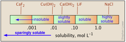
Solubilities are most fundamentally expressed in molar (mol L–1 of solution) or molal (mol kg–1 of water) units. But for practical use in preparing stock solutions, chemistry handbooks usually express solubilities in terms of grams-per-100 ml of water at a given temperature, frequently noting the latter in a superscript. Thus 6.9 20 means 6.9 g of solute will dissolve in 100 mL of water at 20° C. When quantitative data are lacking, the designations "soluble", "insoluble", "slightly soluble", and "highly soluble" are used. There is no agreed-on standard for these classifications, but a useful guideline might be that shown below.
The solubilities of salts in water span a remarkably large range of values, from almost completely insoluble to highly soluble. Moreover, there is no simple way of predicting these values, or even of explaining the trends that are observed for the solubilities of different anions within a given group of the periodic table.
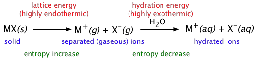
Ultimately, the driving force for dissolution (and for all chemical processes) is determined by the Gibbs free energy change. But because many courses cover solubility before introducing free energy, we will not pursue this here. Dissolution of a salt is conceptually understood as a sequence of the two processes depicted above:
- breakup of the ionic lattice of the solid,
- followed by attachment of water molecules to the released ions.
The first step consumes a large quantity of energy, something that by itself would strongly discourage solubility. But the second step releases a large amount of energy and thus has the opposite effect. Thus the net energy change depends on the sum of two large energy terms (often approaching 1000 kJ/mol) having opposite signs. Each of these terms will to some extent be influenced by the size, charge, and polarizability of the particular ions involved, and on the lattice structure of the solid. This large number of variables makes it impossible to predict the solubility of a given salt. Nevertheless, there are some clear trends for how the solubilities of a series of salts of a given anion (such as hydroxides, sulfates, etc.) change with a periodic table group. And of course, there are a number of general solubility rules — for example, that all nitrates are soluble, while most sulfides are insoluble.
Solubility and temperature
Solubility usually increases with temperature - but not always. This is very apparent from the solubility-vs.-temperature plots shown here. (Some of the plots are colored differently in order to make it easier to distinguish them where they crowd together.) The temperature dependence of any process depends on its entropy change — that is, on the degree to which thermal kinetic energy can spread throughout the system. When a solid dissolves, its component molecules or ions diffuse into the much greater volume of the solution, carrying their thermal energy along with them. So we would normally expect the entropy to increase — something that makes any process take place to a greater extent at a higher temperature.
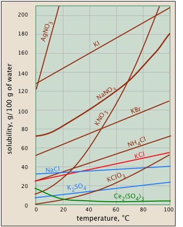
So why does the solubility of cerium sulfate (green plot) diminish with temperature? Dispersal of the Ce3+ and SO42– ions themselves is still associated with an entropy increase, but in this case the entropy of the water decreases even more owing to the ordering of the H2O molecules that attach to the Ce3+ ions as they become hydrated. It's difficult to predict these effects, or explain why they occur in individual cases — but they do happen.
The Importance of Sparingly Soluble Solids
All solids that dissociate into ions exhibit some limit to their solubilities, but those whose saturated solutions exceed about 0.01 mol L–1 cannot be treated by simple equilibrium constants owing to ion-pair formation that greatly complicates their behavior. For this reason, most of what follows in this lesson is limited to salts that fall into the "sparingly soluble" category. The importance of sparingly soluble solids arises from the fact that formation of such a product can effectively remove the corresponding ions from the solution, thus driving the reaction to the right. Consider, for example, what happens when we mix solutions of strontium nitrate and potassium chloride in a 1:2 mole ratio. Although we might represent this process by
\[Sr(NO_3)_{2(aq)}+ 2 KCl_{(aq)}→ SrCl_{(aq)}+ 2 KNO_{3(aq)} \label{1}\]
the net ionic equation
\[Sr^{2+} + 2 NO_3^– + 2 K^+ + 2 Cl^– → Sr^{2+} + 2 NO_3^– + 2 K^+ + 2 Cl^–\]
indicates that no net change at all has taken place! Of course if the solution were than evaporated to dryness, we would end up with a mixture of the four salts shown in Equation \(\ref{1}\), so in this case we might say that the reaction is half-complete. Contrast this with what happens if we combine equimolar solutions of barium chloride and sodium sulfate:
\[BaCl_{2(aq)}+ Na_2SO_{4(aq)}→ 2 NaCl_{(aq)}+ BaSO_{4(s)} \label{2}\]
whose net ionic equation is
\[Ba^{2+} + \cancel{ 2 Cl^–} + \cancel{2 Na^+} + SO_4^{2–} → \cancel{2 Na^+} + \cancel{2 Cl^–} + BaSO_{4(s)}\]
which after canceling out like terms on both sides, becomes simply
\[Ba^{2+} + SO_4^{2– }→ BaSO_{4(s)} \label{3}\]
Because the formation of sparingly soluble solids is "complete" (that is, equilibria such as the one shown above for barium sulfate lie so far to the right), virtually all of one or both of the contributing ions are essentially removed from the solution. Such reactions are said to be quantitative, and they are especially important in analytical chemistry:
- Qualitative analysis: This most commonly refers to a procedural scheme, widely encountered in first-year laboratory courses, in which a mixture of cations (usually in the form of their dissolved nitrate salts) is systematically separated and identified on the basis of the solubilities of their various anion salts such as chlorides, carbonates, sulfates, and sulfides. Although this form of qualitative analysis is no longer employed by modern-day chemists (instrumental techniques such as atomic absorption spectroscopy are much faster and comprehensive), it is still valued as an educational tool for familiarizing students with some of the major classes of inorganic salts, and for developing basic skills relating to observing, organizing, and interpreting results in the laboratory.
- Quantitative gravimetric analysis: In this classical form of chemical analysis, an insoluble salt of a cation is prepared by precipitating it by addition of a suitable anion. The precipitate is then collected, dried, and weighed ("gravimetry") in order to determine the concentration of the cation in the sample. For example, a gravimetric procedure for determining the quantity of barium in a sample might involve precipitating the metal as the sulfate according to Equation \(\ref{3}\) above, using an excess of sulfate ion to ensure complete removal of the barium. This method of quantitative analysis became extremely important in the latter half of the nineteenth century, by which time reasonably accurate atomic weights had become available, and sensitive analytical balances had been developed. It was not until the 1960's that it became largely supplanted by instrumental techniques which were much quicker and accurate. Gravimetric analysis is still usually included as a part of more advanced laboratory instruction, largely as a means of developing careful laboratory technique.
Solubility Products and Equilibria
Some salts and similar compounds (such as some metal hydroxides) dissociate completely when they dissolve, but the extent to which they dissolve is so limited that the resulting solutions exhibit only very weak conductivities. In these salts, which otherwise act as strong electrolytes, we can treat the dissolution-dissociation process as a true equilibrium. Although this seems almost trivial now, this discovery, made in 1900 by Walther Nernst who applied the Law of Mass Action to the dissociation scheme of Arrhenius, is considered one of the major steps in the development of our understanding of ionic solutions.
Using silver chromate as an example, we express its dissolution in water as
\[Ag_2CrO_{4(s)} \rightarrow 2 Ag^+_{(aq)}+ CrO^{2–}_{4(aq)} \label{4a}\]
When this process reaches equilibrium (which requires that some solid be present), we can write (leaving out the "(aq)s" for simplicity)
\[Ag_2CrO_{4(s)} \rightleftharpoons 2 Ag^+ + CrO^{2–}_{4} \label{4b}\]
The equilibrium constant is formally
\[K = \dfrac{[Ag^+]^2[CrO_4^{2–}]}{[Ag_2CrO_{4(s)}]} = [Ag^+]^2[CrO_4^{2–}] \label{5a}\]
But because solid substances do not normally appear in equilibrium expressions, the equilibrium constant for this process is
\[[Ag^+]^2 [CrO_4^{2–}] = K_s = 2.76 \times 10^{–12} \label{5b}\]
Because equilibrium constants of this kind are written as products, the resulting K's are commonly known as solubility products, denoted by \(K_s\) or \(K_{sp}\).
Strictly speaking, concentration units do not appear in equilibrium constant expressions. However, many instructors prefer that students show them anyway, especially when using solubility products to calculate concentrations. If this is done, \(K_s\) in Equation \(\ref{5b}\) would have units of mol3 L–3.
Equilibrium and non-equilibrium in solubility systems
An expression such as [Ag+]2 [CrO42–] in known generally as an ion product — this one being the ion product for silver chromate. An ion product can in principle have any positive value, depending on the concentrations of the ions involved. Only in the special case when its value is identical with Ks does it become the solubility product. A solution in which this is the case is said to be saturated. Thus when
\[[Ag^+]^2 [CrO_4^{2–}] = 2.76 \times 10^{-12}\]
at the temperature and pressure at which this value \(K_s\) of applies, we say that the "solution is saturated in silver chromate".
A solution must be saturated to be in equilibrium with the solid. This is a necessary condition for solubility equilibrium, but it is not by itself sufficient. True chemical equilibrium can only occur when all components are simultaneously present. A solubility system can be in equilibrium only when some of the solid is in contact with a saturated solution of its ions. Failure to appreciate this is a very common cause of errors in solving solubility problems.
Undersaturated and supersaturated solutions
If the ion product is smaller than the solubility product, the system is not in equilibrium and no solid can be present. Such a solution is said to be undersaturated. A supersaturated solution is one in which the ion product exceeds the solubility product. A supersaturated solution is not at equilibrium, and no solid can ordinarily be present in such a solution. If some of the solid is added, the excess ions precipitate out and until solubility equilibrium is achieved.
How to know the saturation status of a solution
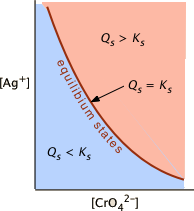
This is just a simple matter of comparing the ion product \(Q_s\) with the solubility product \(K_s\). So for the system
\[Ag_2CrO_{4(s)} \rightleftharpoons 2 Ag^+ + CrO_4^{2–} \label{4ba}\]
a solution in which \(Q_s < K_s\) (i.e., \(K_s /Q_s > 1\)) is undersaturated (blue shading) and the no solid will be present. The combinations of [Ag+] and [CrO42–] that correspond to a saturated solution (and thus to equilibrium) are limited to those described by the curved line. The pink area to the right of this curve represents a supersaturated solution.
A sample of groundwater that has percolated through a layer of gypsum (CaSO4, Ks = 4.9E–5 = 10–4.3) is found to have be 8.4E–5 M in Ca2+ and 7.2E–5 M in SO42–. What is the equilibrium state of this solution with respect to gypsum?
Solution
The ion product
\[Q_s = (8.4 \times 10^{–5})(7.2 \times 10^{-5}) = 6.0 \times 10^{–4}\]
exceeds \(K_s\), so the ratio Ks /Qs > 1 and the solution is supersaturated in CaSO4.
How are solubilities determined?
There are two principal methods, neither of which is all that reliable for sparingly soluble salts:
- Evaporate a saturated solution of the solid to dryness, and weigh what's left.
- Measure the electrical conductivity of the saturated solution, which will be proportional to the concentrations of the ions.
How Solubilities relate to solubility products
The solubility (by which we usually mean the molar solubility) of a solid is expressed as the concentration of the "dissolved solid" in a saturated solution. In the case of a simple 1:1 solid such as AgCl, this would just be the concentration of Ag+ or Cl– in the saturated solution. However, for a more complicated stoichiometry such as as silver chromate, the solubility would be only one-half of the Ag+ concentration.
For example, let us denote the solubility of Ag2CrO4 as \(S\) mol L–1. Then for a saturated solution, we have
- \([Ag^+] = 2S\)
- \( [CrO_4^{2–}] = S\)
Substituting this into Equation \(\ref{5b}\) above,
\[(2S)^2 (S) = 4S^3 = 2.76 \times 10^{–12}\]
\[S= \left( \dfrac{K_s}{4} \right)^{1/3} = (6.9 \times 10^{-13})^{1/3} = 0.88 \times 10^{-4} \label{6a}\]
thus the solubility is \(8.8 \times 10^{–5}\; M\).
Note that the relation between the solubility and the solubility product constant depends on the stoichiometry of the dissolution reaction. For this reason it is meaningless to compare the solubilities of two salts having the formulas \(A_2B\) and \(AB_2\), on the basis of their \(K_s\) values.
It is meaningless to compare the solubilities of two salts having different formulas on the basis of their \(K_s\) values.
under these conditions.
Solution
moles of solute in 100 mL; S = 0.0016 g / 78.1 g/mol = 2.05E-5 mol
S = 2.05E–5 mol/0.100 L = 2.05E-4 M
Ks = [Ca2+][F–]2 = (S)(2S)2 = 4 × (2.05E–4)3 = 3.44E–11
Estimate the solubility of La(IO3)3 and calculate the concentration of iodate in equilibrium with solid lanthanum iodate, for which Ks = 6.2 × 10⁻¹².
Solution
The equation for the dissolution is
\[La(IO_3)_3 \rightleftharpoons La^{3+ }+ 3 IO_3^–\]
If the solubility is S, then the equilibrium concentrations of the ions will be
[La3+] = S and [IO3–] = 3S. Then Ks = [La3+][IO3–]3 = S(3S)3 = 27S4
27S4 = 6.2 × 10⁻¹², S = ( ( 6.2 ÷ 27) × 10–12 )¼ = 6.92 × 10⁻⁴ M
[IO3–] = 3S = 2.08 × 10⁻⁵ (M)
Cadmium is a highly toxic environmental pollutant that enters wastewaters associated with zinc smelting (Cd and Zn commonly occur together in ZnS ores) and in some electroplating processes. One way of controlling cadmium in effluent streams is to add sodium hydroxide, which precipitates insoluble Cd(OH)2 (Ks = 2.5E–14). If 1000 L of a certain wastewater contains Cd2+ at a concentration of 1.6E–5 M, what concentration of Cd2+ would remain after addition of 10 L of 4 M NaOH solution?
Solution
As with most real-world problems, this is best approached as a series of smaller problems, making simplifying approximations as appropriate.
Volume of treated water: 1000 L + 10 L = 1010 L
Concentration of OH– on addition to 1000 L of pure water:
(4 M) × (10 L)/(1010 L) = .040 M
Initial concentration of Cd2+ in 1010 L of water:
(1.6E–5 M) x (100/101) ≈ 1.6E–5 M
The easiest way to tackle this is to start by assuming that a stoichiometric quantity of Cd(OH)2 is formed — that is, all of the Cd2+ gets precipitated.
| Concentrations | [Cd2+], M | [OH–], M |
|---|---|---|
| initial | 1.6E–5 | 0.04 |
| change | –1.6E–5 | –3.2E–5 |
| final: | 0 | 0.04 – 3.2E–5 ≈ .04 |
Now "turn on the equilibrium" — find the concentration of Cd2+ that can exist in a 0.04M OH– solution:
| Concentrations | [Cd2+], M | [OH–], M |
|---|---|---|
| initial | o | 0.04 |
| change | +x | +2x |
| at equilibrium | x | 0.04 + 2x ≈ .04 |
Substitute these values into the solubility product expression:
\[Cd(OH)_{2(s) } = [Cd^{2+}] [OH^–]^2 = 2.5 \times 10^{–14}\]
\[[Cd^{2+}] = \dfrac{2.5 \times 10^{–14}}{ 16 \times 10^{–4}} = 1.6 \times 10^{–13}\; M\]
Note that the effluent will now be very alkaline:
\[pH = 14 + \log 0.04 = 12.6\]
so in order to meet environmental standards an equivalent quantity of strong acid must be added to neutralize the water before it is released.
All Just a Simplification of Reality
The simple relations between Ks and molar solubility outlined above, and the calculation examples given here, cannot be relied upon to give correct answers. Some of the reasons for this are explained in Part 2 of this lesson, and have mainly to do with incomplete dissociation of many salts and with complex formation in the presence of anions such as Cl– and OH–. The situation is nicely described in the article What Should We Teach Beginners about Solubility and Solubility Products? by Stephen Hawkes (J Chem Educ.1998 75(9) 1179-81). See also the earlier article by Meites, Pode and Thomas Are Solubilities and Solubility Products Related?(J Chem Educ. 1966 43(12) 667-72).
It turns out that solubility equilibria more often than not involve many competing processes and their rigorous treatment can be quite complicated. Nevertheless, it is important that students master these over-simplified examples. However, it is also important that they are not taken too seriously!
The Common Ion Effect
It has long been known that the solubility of a sparingly soluble ionic substance is markedly decreased in a solution of another ionic compound when the two substances have an ion in common. This is just what would be expected on the basis of the Le Chatelier Principle; whenever the process
\[CaF_{2(s)} \rightleftharpoons Ca^{2+} + 2 F^– \label{7}\]
is in equilibrium, addition of more fluoride ion (in the form of highly soluble NaF) will shift the composition to the left, reducing the concentration of Ca2+, and thus effectively reducing the solubility of the solid. We can express this quantitatively by noting that the solubility product expression
\[[Ca^{2+}][F^–]^2 = 1.7 \times 10^{–10} \label{8}\]
must always hold, even if some of the ionic species involved come from sources other than CaF2(s). For example, if some quantity x of fluoride ion is added to a solution initially in equilibrium with solid CaF2, we have
- \([Ca^{2+}] = S\)
- \([F^–] = 2S + x\)
so that
\[K_s = [Ca^{2+}][ F^–]^2 = S (2S + x)^2 . \label{9a}\]
\[K_s ≈ S x^2 \]
or
\[S ≈ \dfrac{K_s}{x^2} \label{9b}\]
University-level students should be able to derive these relations for ion-derived solids of any stoichiometry.
The plots shown below illustrate the common ion effect for silver chromate as the chromate ion concentration is increased by addition of a soluble chromate such as \(Na_2CrO_4\).
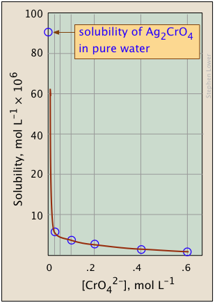
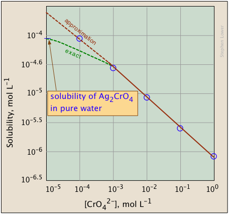
What's different about the plot on the right? If you look carefully at the scales, you will see that this one is plotted logarithmically (that is, in powers of 10.) Notice how a much wider a range of values can display on a logarithmic plot. The point of showing this pair of plots is to illustrate the great utility of log-concentration plots in equilibrium calculations in which simple approximations (such as that made in Equation \(\ref{9b}\) can yield straight-lines within the range of values for which the approximation is valid.
Calculate the solubility of strontium sulfate (Ks = 2.8 × 10⁻⁷) in
- pure water and
- in a 0.10 mol L–1 solution of \(Na_2SO_4\).
\[S = \sqrt{K_s} = \sqrt{ 2.8 \times 10^{–7} } = 5.3 \times 10^{–4}\]
(b) In 0.10 mol L–1 Na2SO4, we have
= [Sr2+][SO42–] = S × (0.10 + S) = 2.8 × 10⁻⁷Because S is negligible compared to 0.10 M, we make the approximation
= [Sr2+][SO42–] ≈ S × (0.10 M) = 2.8 × 10⁻⁷so
This is roughly 100 times smaller than the result from (a).
Selective Precipitation and Separations
Differences in solubility are widely used to selectively remove one species from a solution containing several kinds of ions.
The solubility products of AgCl and Ag2CrO4 are 1.8E–10 and 2.0E–12, respectively. Suppose that a dilute solution of AgNO3 is added dropwise to a solution containing 0.001M Cl– and 0.01M CrO42–.
- Which solid, AgCl or Ag2CrO4, will precipitate first?
- What fraction of the first anion will have been removed when the second just begins to precipitate? Neglect any volume changes.
Solution
The silver ion concentrations required to precipitate the two salts are found by substituting into the appropriate solubility product expressions:
- to precipitate AgCl: [Ag+] = 1.8E-10 / .001 = 1.8E-7 M
- to precipitate Ag2CrO4: [Ag+] = (2.0E-12 / .01)½ = 1.4E–5 M
The first solid to form as the concentration of Ag+ increases will be AgCl. Eventually the Ag+ concentration reaches 1.4E-5 M and Ag2CrO4 begins to precipitate. At this point the concentration of chloride ion in the solution will be 1.3E-5 M which is about 13% of the amount originally present.
The preceding example is the basis of the Mohr titration of chloride by Ag+, commonly done to determine the salinity of water samples. The equivalence point of this precipitation titration occurs when no more AgCl is formed, but there is no way of observing this directly in the presence of the white AgCl which is suspended in the container. Before the titration is begun, a small amount of K2CrO4 is added to the solution. Ag2CrO4 is red-orange in color, so its formation, which signals the approximate end of AgCl precipitation, can be detected visually.
Competing Equilibria involving solids
Solubility expression are probably the exception rather than the rule. Such equilibria are often in competition with other reactions with such species as H+or OH–, complexing agents, oxidation-reduction, formation of other sparingly soluble species or, in the case of carbonates and sulfites, of gaseous products. The exact treatments of these systems can be extremely complicated, involving the solution of large sets of simultaneous equations. For most practical purposes it is sufficient to recognize the general trends, and to carry out approximate calculations.
Salts of weak acids are soluble in strong acids, but strong acids will not dissolve salts of strong acids
The solubility of a sparingly soluble salt of a weak acid or base will depend on the pH of the solution. To understand the reason for this, consider a hypothetical salt MA which dissolves to form a cation M+ and an anion A–which is also the conjugate base of a weak acid HA. The fact that the acid is weak means that hydrogen ions (always present in aqueous solutions) and M+ cations will both be competing for the A–:
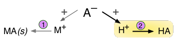
The weaker the acid HA, the more readily will reaction  take place, thus gobbling up A– ions. If an excess of H+ is made available by addition of a strong acid, even more A– ions will be consumed, eventually reversing reaction
  , causing the solid to dissolve.
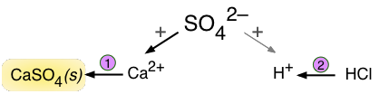
In  , for example, sulfate ions react with calcium ions to form insoluble CaSO4. Addition of a strong acid such as HCl (which is totally dissociated ) has no effect because CaCl2 is soluble. Although H+ can protonate some SO42– ions to form hydrogen sulfate ("bisulfate") HSO4–, this ampholyte acid is too weak to reverse by drawing a significant fraction of sulfate ions out of CaSO4(s).
Calculate the concentration of aluminum ion in a solution that is in equilibrium with aluminum hydroxide when the pH is held at 6.0.
The equilibria are
\[Al(OH)_3 \rightleftharpoons Al^{3+} + 3 OH^–\]
with
\[K_s = 1.4 \times 10^{–34}\]
and
\[H_2O \rightleftharpoons H^+ + OH^–\]
with
\[K_w = 1 \times 10^{–14}\]
Substituting the equilibrium expression for the second of these into that for the first, we obtain
\[[OH^–]^3 = \left( \dfrac{K_w}{ [H^+]}\right)^3 = \dfrac{K_s}{[Al^{3+}]}\]
(1.0 × 10⁻¹⁴) / (1.0 × 10⁻⁶)3 = (1.4 × 10⁻²⁴) / [Al3+]
from which we find
\[[Al^{3+}] = 1.4 \times 10^{–10}\; M\]
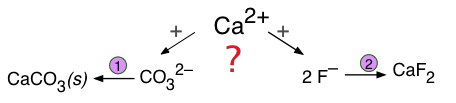
Formation of a Competing Precipitate
If two different anions compete with a single cation to form two possible precipitates, the outcome depends not only on the solubilities of the two solids, but also on the concentrations of the relevant ions.
These kinds of competitions are especially important in groundwaters, which acquire solutes from various sources as they pass through sediment layers having different compositions. As the following example shows, competing equilibria of these kinds are very important for understanding geochemical processes involving the formation and transformation of mineral deposits.
Suppose that groundwater containing 0.001M F– and 0.0018M CO32– percolates through a sediment containing calcite, CaCO3. Will the calcite be replaced by fluorite, CaF2?
The two solubility equilibria are
\[\ce{CaCO3 <=> Ca^{2+} + CO3^{2–} \quad K_s = 10^{–8.1}\]
\[\ce{CaF2 <=> Ca^{2+} + 2 F^{–} \quad K_s = 10^{–10.4}\]
Solution:
The equilibrium between the two solids and the two anions is
\[CaCO_3 + 2 F^–\rightleftharpoons CaF_2 + CO_3^{2–}\]
This is just the sum of the dissolution reaction for CaCO3 and the reverse of that for CaF2, so the equilibrium constant is
\[K = \dfrac{[CO_3^{2–}]}{ [F^–]^2} = \dfrac{10^{–8.1}}{ 10^{–10.4}} = 200\]
That is, the two solids can coexist only if the reaction quotient Q ≤ 200. Substituting the given ion concentrations we find that
\[Q = \dfrac{0.0018}{0.0012} = 1800\]
Since Q>K, we can conclude that the calcite will not change into fluorite.
Complex Ion Formation
Most transition metal ions possess empty d orbitals that are sufficiently low in energy to be able to accept electron pairs from electron donors from cations, resulting in the formation of a covalently-bound complex ion. Even neutral species that have a nonbonding electron pair can bind to ions in this way. Water is an active electron donor of this kind, so aqueous solutions of ions such as Fe3+(aq) and Cu2+(aq) exist as the octahedral complexes Fe(H2O)63+ and Cu(H6O)62+, respectively.
Many of the remarks made above about the relation between Ks and solubility also apply to calculations involving complex formation. See Stephen Hawkes' article Complexation Calculations are Worse Than Useless ("... to the point of absurdity...and should not be taught" in introductory courses.) (J Chem Educ. 1999 76(8) 1099-1100). However, it is very important that you understand the principles outlined in this section.
H2O is only one possible electron donor; NH3, CN– and many other species (known collectively as ligands) possess lone pairs that can occupy vacantd orbitals on a metallic ion. Many of these bind much more tightly to the metal than does H2O, which will undergo displacement and substitution by one or more of these ligands if they are present in sufficiently high concentration.
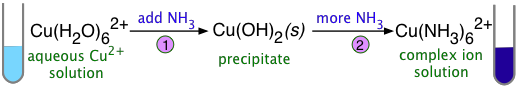
If a sparingly soluble solid is placed in contact with a solution containing a ligand that can bind to the metal ion much more strongly than H2O, then formation of a complex ion will be favored and the solubility of the solid will be greater. Perhaps the most commonly seen example of this occurs when ammonia is added to a solution of copper(II) nitrate, in which the Cu2+(aq) ion is itself the complex hexaaquo complex ion shown at the left:
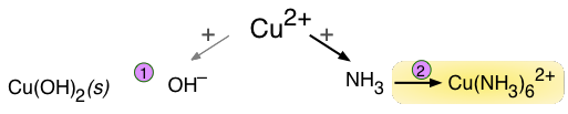
Because ammonia is a weak base, the first thing we observe is formation of a cloudy precipitate of Cu(OH)2 in the blue solution. As more ammonia is added , this precipitate dissolves, and the solution turns an intense deep blue, which is the color of hexamminecopper(II) and the various other related species such as Cu(H2O)5(NH3)2+, Cu(H2O)4(NH3)22+, etc.
In many cases, the complexing agent and the anion of the sparingly soluble salt are identical. This is particularly apt to happen with insoluble chlorides, and it means that addition of chloride to precipitate a metallic ion such as Ag+ will produce a precipitate at first, but after excess Cl– has been added the precipitate will redissolve as complex ions are formed.
Some important solubility systems
In this section, we discuss solubility equilibria that relate to some very commonly-encountered anions of metallic salts. These are especially pertinent to the kinds of separations that most college students are required to carry out (and understand!) in their first-year laboratory courses.
Solubility of oxides and hydroxides
Metallic oxides and hydroxides both form solutions containing OH– ions. For example, the solubilities of the [sparingly soluble] oxide and hydroxide of magnesium are represented by
\[Mg(OH)_{2(s)} → Mg^{2+} + 2 OH^– \label{10}\]
\[MgO_{(S)} + H_2O → Mg^{2+} + 2 OH^– \label{11}\]
If you write out the solubility product expressions for these two reactions, you will see that they are identical in form and value.
Recall that pH = –log10[H+], so that [H+] = 10–pH.
One might naïvely expect that the dissolution of an oxide such as MgO would yield as one of its products the oxide ion O2+. But the oxide ion is such a strong base that it grabs a proton from water, forming two hydroxide ions instead:
\[O^{2+} + H_2O → 2 OH^–\]
This is an example of the rule that the hydroxide ion is the strongest base that can exist in aqueous solution.2" is an equilibrium mixture of hydrated CO2molecules and carbonic acid. To keep things as simple as possible, we will not distinguish between them in what follows, and just use the formula H2CO3 to represent the two species collectively.
The other Group 2 metals, especially Mg, along with iron and several other transition elements are also found in carbonate sediments. When rain falls through the air, it absorbs atmospheric carbon dioxide, a small portion of which reacts with the water to form carbonic acid. Thus all pure water in contact with the air becomes acidic, eventually reaching a pH of 5.6.
As noted above, the equilibrium between bicarbonate and carbonate ions depends on the pH. Since the pH scale is logarithmic, it makes sense (and greatly simplifies the construction of the plot) to employ a log scale for the concentrations. The plot shown below corresponds to a total carbonate-system concentration of 10–3 M, which is representative of many ground waters. For river and lake waters, 10–5 M would be more typical; this would simply shift the curves downward without affecting their shapes.
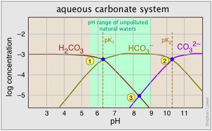
Points 1 and 2 where adjacent curves overlap correspond to the two pK's. Recall that when the pH is the same as the pK, the concentrations of the two conjugate species are identical and half of the total system concentration. This places the crossover points at log 0.5 = –0.3 below the system concentration level.
A 10–3 M solution of sodium bicarbonate would have a pH denoted by point 3, with [H2CO3] and [CO32–] constituting only 1% (10–5 M) of the system. This corresponds to the equilibrium
\[2 HCO_3^– \rightleftharpoons H_2CO_3 + CO_3^{2–}\]
Carbonates act as bases and, as such, react with acids. Thus, the portion of the global water cycle that transports carbon from the air into natural waters constitutes a gigantic acid-base reaction that yields hydrogen carbonate ions, commonly referred to as bicarbonate. The natural waters that result have pH values between 6 and 10 and are essentially solutions of bicarbonates.
Limestone caves and sinkholes
When rainwater permeates into the soil, it can become even more acidic owing to the additional CO2 produced by soil organisms. Also, the deeper the water penetrates, the greater its hydrostatic pressure and the more CO2 it can hold, further increasing its acidity. If this water then works its way down through the fissures and cracks within a limestone layer, it will dissolve some of limestone, leaving void spaces which may eventually grow into limestone caves or form sinkholes that can swallow up cars or houses.
A well-known feature of limestone caves is the precipitated carbonate formations that decorate the ceilings and floors. These are known as stalactites and stalagmites, respectively. When water emerges from the ceiling of a cave that is open to the atmosphere, some of the excess CO2 it contains is released as it equilibrates with the air. This raises its pH and thus reduces the solubility of of the carbonates, which precipitate as stalactites. Some of the water remains supersaturated and does not precipitate until it drips to the cave floor, where it builds up the stalagmite formations.
Hard Water
This term refers to waters that, through contact with rocks and sediments in lakes, streams, and especially in soils (groundwaters), have acquired metallic cations such as Ca2+, Mg2+, Fe2+, Fe3+, Zn2+ Mn2+, etc. Owing to the ubiquity of carbonate sediments, the compensating negative charge is frequently supplied by the bicarbonate ion HCO3–, but other anions such as SO42–, F–, Cl–, PO43– and SiO42– may also be significant.
Solid bicarbonates are formed only by Group 1 cations and all are readily soluble in water. But because HCO3– is amphiprotic, it can react with itself to yield carbonate:
\[2 HCO_3^– → H_2O + CO_3^[2–} + CO_{2(g)}\]
If bicarbonate-containing water is boiled, the CO2 is driven off, and the equilibrium shifts to the right, causing any Ca2+ or similar ions to form a cloudy precipitate. If this succeeds in removing the "hardness cations", the water has been "softened". Such water is said to possess carbonate hardness, sometimes known as "temporary hardness". Waters in which anions other than HCO3– predominate cannot be softened by boiling, and thus possess non-carbonate hardness or "permanent hardness".
Hard waters present several kinds of problems, both in domestic and industrial settings:
- Waters containing dissolved salts leave solid deposits when they evaporate. Residents of areas having hard water (about 85 percent of the U.S.) notice evaporative deposits on shower walls, in teakettles, and on newly-washed windows, glassware, and vehicles.
- Much more seriously from an economic standpoint, evaporation of water in boilers used for the production of industrial steam leaves coatings on the heat exchanger surfaces that impede the transfer of heat from the combustion chamber, reducing the thermal transfer efficiency. The resultant overheating of these surfaces can lead to their rupture, and in the case of high-pressure boilers, to disastrous explosions. In the case of calcium and magnesium carbonates, the process is exacerbated by the reduced solubility of these salts at high temperatures. Removal of boiler scales is difficult and expensive.
- Municipal water supplies in hard-water areas tend to be supersaturated in hardness ions. As this water flows through distribution pipes and the plumbing of buildings, these ions often tend to precipitate out on their interior surfaces. Eventually, this scale layer can become thick enough to restrict or even block the flow of water through the pipes. When scale deposits within appliances such as dishwashers and washing machines, it can severely degrade their performance.
- Cations of Group 2 and above react with soaps, which are sodium salts of fatty acids such as stearic acid, C17H35COOH. The sodium salts of such acids are soluble in water, which allows them to dissociate and act as surfactants:
\[C_{17}H_{35}COONa → C_{17}H_{35}COO^– Na^+\]
but the presence of polyvalent ions causes them to form precipitates
\[2 C_{17}H_{35}COO^– + Ca^{2+} → (C_{17}H_{35}COO^–)_2Ca_{(s)}\]
Calcium stearate is less dense than water, so it forms a scum that floats on top of the water surface; anyone who lives in a hard-water area is likely familiar with the unsightly "bathtub rings" it leaves around the high-water mark or the shower-wall stains.
Solubility Complications
All heterogeneous equilibria, on close examination, are beset with complications. But solubility equilibria are somewhat special in that there are more of them. Back in the days when the principal reason for teaching about solubility equilibria was to prepare chemists to separate ions in quantitative analysis procedures, these problems could be mostly ignored. But now that the chemistry of the environment has grown in importance — especially that relating to the ocean and natural waters — there is more reason for chemical scientists to at least know about the limitations of simple solubility products. This section will offer a quick survey of the most important of these complications, while leaving their detailed treatment to more advanced courses.
Tabulated Ks values are notoriously unreliable
Many of the \(K_s\) values found in tables were determined prior to 1940 (some go back to the 1880s!) at a time before highly accurate methods became available. Especially suspect are many of those for highly insoluble salts which are more difficult to measure. A table showing the variations in \(K_{sp}\) values for the same salts among ten textbooks was published by Clark and Bonikamp in J Chem Educ. 1998 75(9) 1183-85.A good An example that used a variety of modern techniques to measure the solubility of silver chromate was published by A.L. Jones et al in the Australian J. of Chemistry, 1971 24 2005-12.
Generations of chemistry students have amused themselves by comparing the disparate Ks values to be found in various textbooks and table. In some cases, they differ by orders of magnitude. There are several reasons for this in addition to the ones described in detail further on.
- The most direct methods of measuring solubilities tend to not be very accurate for sparingly soluble salts. Two-significant figure precision is about the best one can hope in a single measurement.
- Many insoluble salts can exist in more than one crystalline form (polymorphs), and in some cases also as amorphous solids. Precipitation under different conditions (in the presence of different ions, at different temperatures, etc.) can yield different or mixed polymorphs.
- Other ions present in the solution can often get incorporated into the crystalline solid, usually replacing an ion of similar size (substitutional solid solutions). When this happens, it is no longer valid to write the equilibrium condition as a simple "product". This is very common in mineral deposits, and an important consideration in geochemistry,
Most salts are not Completely Dissociated in Water
The dissolution of cadmium iodide is water is commonly represented as
\[CdI_{2(s)} → Cd^{2+} + 2 I^–\]
Firstly, they combine to form neutral, largely-covalent molecular species:
\[Cd^{2+}_{(aq)} + 2 I^–_{(aq)} → CdI_{2(aq)}\]
This non-ionic form accounts for 78% of the Cd present in the solution! In addition, they form a molecular ion \(CdI^–_{(aq)}\) according to the following scheme:
| \(CdI_{2(s)} \rightleftharpoons Cd^{2+} + 2 I^–\) | \(K_1 = 10^{–3.9}\) |
| \(Cd^{2+} + I^– \rightleftharpoons CdI^+\) | \(K_2= 10^{+2.3}\) |
| \(CdI2_{(s)} \rightleftharpoons CdI^++ I^–\) | \(K = 10^{–1.6} = 0.023\) |
The data shown Tables \(\PageIndex{1}\) and \(\PageIndex{2}\) are taken from the article Salts are Mostly NOT Ionized by Stephen Hawkes: 1996 J Chem Educ. 73(5) 421-423. This fact was stated by Arrhenius in 1887, but has been largely ignored and is rarely mentioned in standard textbooks.
As a consequence, the concentration of "free" Cd2+(aq) in an aqueous cadmium iodide solution is only about 2% of the value you would calculate by taking K1 as the solubility product. The principal component of such as solution is actually [covalently-bound] CdI2(aq). It turns out that many salts, especially those of metals beyond Group 2, are similarly only partially ionized in aqueous solution:
| salt | molarity | % cation | other species |
|---|---|---|---|
| KCl | 0.52 | 95 | KCl(aq) 5% |
| MgSO4 | 0.04 | 58 | MgSO4(aq) 42% |
| CaCl2 | 0.44 | 70 | CaCl+(aq) 30% |
| CuSO4 | 0.045 | 56 | CuSO4(aq) 44% |
| CdI2 | 0.50 | 2 | CdI2(aq) 76%, CdI–(aq) 22% |
| FeCl3 | 0.1 | 10 | FeCl2+(aq) 42%, FeCl2(aq) 40%, FeOH2+(aq) 6%, Fe(OH)2+(aq) 2% |
If you are enrolled in an introductory course and do not plan on taking more advanced courses in chemistry or biochemistry, you can probably be safe in ignoring this, since your instructor and textbook likely do so. However, if you expect to do more advanced work or teach, you really should take note of these points, since few textbooks mention them.
Formation of Hydrous Complexes
Transition metal ions form a large variety of complexes with H2O and OH–, both of which have electron-pairs available to coordinate with the central ion. This gives rise to a large variety of soluble species that are in competition with an insoluble solid. Because of this, a single equilibrium constant (solubility product) cannot describe the behavior of a solid such as Fe(OH)3, which we summarize here as an example.
Aquo complexes: The electrostatic field of the positively-charged metal ion enhances the acidic nature of these H2O molecules, encouraging them to shed a proton and leaving OH– groups in their place.
\[Fe(H_2O)_6^{3+} → Fe(H_2O)_5(OH)^{2+}+H^+\]
This is just the first of a series of similar reactions, each one having a successively smaller equilibrium constant:
\[Fe(H_2O)_5(OH)^{2+}→ Fe(H_2O)_4(OH)_2^+→ Fe(H_2O)_3(OH)_3 → Fe(H_2O)_2(OH)_4^-\]
Hydroxo complexes: But there's more: when the hydroxide ion acts as a ligand, it gives rise to a series of hydroxo complexes, of which the insoluble Fe(OH)3 can be considered a member:
| Fe3+ + 3 OH– → Fe(OH)3(s) | 1/Ks = 1038 |
| Fe3+ + H2O → Fe(OH)2+ + H+ | K = 10–2.2 |
| Fe3+ + 2H2O → FeOH+ + 2H+ | K = 10–6.7 |
| Fe3+ + 4H2O → Fe(OH)4– + 4H+ | K = 10–23 |
| 2Fe3+ + 2H2O → Fe2(OH)24+ + 2H+ | K = 10–2.8 |
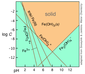
The equilibria listed above all involve H+ and OH– ions, and are therefore pH dependent, as illustrated by the straight lines in the plot, whose slopes reflect the pH dependence of the corresponding ionic species. At any given pH, the equilibrium with solid Fe(OH)3 is controlled by the ionic species having the highest concentration at any given pH. The corresponding lines in the plot therefore delineate the region (indicated by the orange shading) at which the solid can exist.
Ionic interactions: The "non-common ion effect"
A sparingly-soluble salt will be more soluble in a solution that contains non-participating ions. This is just the opposite of the common ion effect, and it might at first seem rather counter-intuitive: why would adding more ions of any kind make a salt more likely to dissolve?
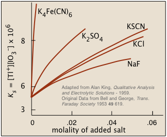
Figure \(\PageIndex{2}\): Solubility of thallium iodate in solutions containing dissolved salts
A clue to the answer can be found in another fact: the higher the charge of the foreign ion, the more pronounced is the effect. This tells us that inter-ionic (and thus electrostatic) interactions must play a role. The details are rather complicated, but the general idea is that all ions in solution, besides possessing tightly-held waters of hydration, tend to attract oppositely-charged ions ("counter-ions") around them. This "atmosphere" of counterions is always rather diffuse, but much less so (and more tightly bound) when one or both kinds of ions have greater charges. From a distance, these ion-counterion bodies appear to be almost electrically neutral, which keeps them from interacting with each other (as to form a precipitate).
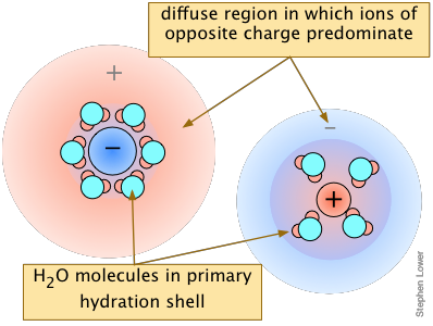
The overall effect is to reduce the concentrations of the less-shielded ions that are available to combine to form a precipitate. We say that the thermodynamically-effective concentrations of these ions are less than their "analytical" concentrations. Chemists refer to these effective concentrations as ionic activities, and they denote them by curly brackets {Ag+} as opposed to square brackets [Ag+] which refer to the nominal or analytical concentrations.
Although the concentrations of ions in equilibrium with a sparingly soluble solid are so low that they are essentially the same as the activities, the presence of other ions at concentrations of about 0.001M or greater can materially reduce the activities of the dissolution products, permitting the solubilities to be greater than what simple equilibrium calculations would predict.
Measured solubilities are averages and depend on size
The heterogeneous nature of dissolution reactions leads to a number of peculiar effects relating to the nature of equilibria involving surfaces. These arise from the fact that the tendency of a crystalline solid to dissolve will depend on the particular face or location from which dissolution occurs. Since all crystals present a variety of faces to the solution, a measured Ks is really an average of values for these various faces.
And because many salts can exhibit different external shapes depending on the conditions under which they are formed, solubility products are similarly dependent on these conditions.
Very small crystals are more soluble than big ones
Molecules or ions that are situated on edges or corners are less strongly bound to the remainder of the solid than those on plane surfaces, and will consequently tend to dissolve more readily. Thus the leftmost face in the schematic lattice below will have more edge-bound molecular units than the other two, and this face (11) will be more soluble.
This means, among other things, that smaller crystals, in which the ratio of edges and corners is greater, will tend to have greater Ks values than larger ones. As a consequence, smaller crystals will tend to disappear in favor of larger ones. Practical use is sometimes made of this when the precipitate initially formed in a chemical analysis or separation is too fine to be removed by filtration. The suspension is held at a high temperature for several hours, during with time the crystallites grow in size. This procedure is sometimes referred to as digestion.
Formation of supersaturated solutions
Contrary to what you may have been taught, precipitates do not form when the ion concentration product reaches the solubility product of a salt in a solution that is pure and initially unsaturated; to form a precipitate from a homogeneous solution, a certain degree of supersaturation is required. The extent of supersaturation required to initiate precipitation can be surprisingly great. Thus formation of barium sulfate BaSO4 by combining the two kinds of ions does not occur until Qs exceeds Ks by a factor of 160 or more. In part, this reflects the fact that precipitation proceeds by a series of reactions beginning with formation of an ion-pair which eventually becomes an ion cluster:
Ba2+ + SO42– → (BaSO4)0 → (BaSO4)20 → (BaSO4)30 → etc.
Owing to their overall neutrality, these aggregates are not stabilized by hydration, so they are more likely to break up than not. But a few may eventually survive until they are large enough (but still submicroscopic in size) to serve as precipitation nuclei.
Many substances other than salts form supersaturated solutions, and some salts form them more readily than others. Supersaturated solutions are easily made by dissolving the solid to near its solubility limit in a warmed solvent, and then letting it cool.
Ks) and are inherently unstable; dropping a "seed" crystal of the solid into such a solution will usually initiate rapid precipitation. But as is explained below, even a tiny dust particle may be enough. An old chemist's trick is to use the tip of a glass stirring rod to scrape the inner surface of a container holding a supersaturated solution; the minute particles of glass that are released presumably serve as precipitation nuclei.
The nucleation problem: precipitation is [theoretically] impossible!
Any process in which a new phase forms within an existing homogeneous phase is beset by the nucleation problem: the smallest of these new phases — raindrops forming in air, tiny bubbles forming in a liquid at its boiling point — are inherently less stable than larger ones, and therefore tend to disappear. The same is true of precipitate formation: if smaller crystals are more soluble, then how can the tiniest, first crystal, form at all?
In any ionic solution, small clumps of oppositely-charged ions are continually forming by ordinary collisional processes. The smallest of these aggregates possess a higher free energy than the isolated solvated ions, and they rapidly dissociate. Occasionally, however, one of these proto-crystallites reaches a critical size whose stability allows it to remain intact long enough to serve as a surface (a "nucleus") onto which the deposition of additional ions can lead to still greater stability. At this point, the process passes from the nucleation to the growth stage.
Theoretical calculations predict that nucleation from a perfectly homogeneous solution is a rather unlikely process; tenfold supersaturation should produce only one nucleus per cm3 per year. Most nucleation is therefore believed to occur heterogeneously on the surface of some other particle, possibly a dust particle. The efficiency of this process is critically dependent on the nature and condition of the surface that gives rise to the nucleus.