11: Brownian Motion

Last updated
Save as PDF

Page ID: 294320

\( \newcommand{\vecs}[1]{\overset { \scriptstyle \rightharpoonup} {\mathbf{#1}} } \) \( \newcommand{\vecd}[1]{\overset{-\!-\!\rightharpoonup}{\vphantom{a}\smash {#1}}} \)\(\newcommand{\id}{\mathrm{id}}\) \( \newcommand{\Span}{\mathrm{span}}\) \( \newcommand{\kernel}{\mathrm{null}\,}\) \( \newcommand{\range}{\mathrm{range}\,}\) \( \newcommand{\RealPart}{\mathrm{Re}}\) \( \newcommand{\ImaginaryPart}{\mathrm{Im}}\) \( \newcommand{\Argument}{\mathrm{Arg}}\) \( \newcommand{\norm}[1]{\| #1 \|}\) \( \newcommand{\inner}[2]{\langle #1, #2 \rangle}\) \( \newcommand{\Span}{\mathrm{span}}\) \(\newcommand{\id}{\mathrm{id}}\) \( \newcommand{\Span}{\mathrm{span}}\) \( \newcommand{\kernel}{\mathrm{null}\,}\) \( \newcommand{\range}{\mathrm{range}\,}\) \( \newcommand{\RealPart}{\mathrm{Re}}\) \( \newcommand{\ImaginaryPart}{\mathrm{Im}}\) \( \newcommand{\Argument}{\mathrm{Arg}}\) \( \newcommand{\norm}[1]{\| #1 \|}\) \( \newcommand{\inner}[2]{\langle #1, #2 \rangle}\) \( \newcommand{\Span}{\mathrm{span}}\)\(\newcommand{\AA}{\unicode[.8,0]{x212B}}\)

Brownian motion refers to the random motions of small particles under thermal excitation in solution first described by Robert Brown (1827),¹ who with his microscope observed the random, jittery spatial motion of pollen grains in water. This phenomenon is intrinsically linked with diffusion. Diffusion is the macroscopic realization of the Brownian motion of molecules within concentration gradients. The theoretical basis for this relationship was described by Einstein in 1905,² and Jean Perrin³ provided the detailed experiments that confirmed his predictions.
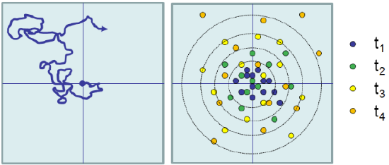
Since the motion of any one particle is unique, the Brownian motion must be described statistically. We observe that the mean-squared displacement of a particle averaged over many measurements grows linearly with time, just as with diffusion.

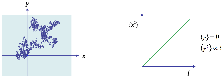
The proportionality factor between mean-squared displacement and time is the diffusion constant in Fick’s Second Law. As for diffusion, the proportionality factor depends on dimensionality. In 1D, if \(\langle x^2(t) \rangle /t = 2D \) then in 3D \( \langle r^2(t) \rangle /t = 6D \), where D is the diffusion constant.

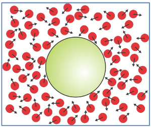Brownian motion is a property of molecules at thermal equilibrium. It applies to a larger particle (i.e., a protein) experiencing an imbalance of many microscopic forces exerted by many much small molecules of the surroundings (i.e., water). The thermal agitation originates by partitioning the kinetic energy of the system on average as k_BT/2 per degree of freedom. Free diffusion implies motion which is only limited by kinetic energy.

Brownian motion applies to a specific range of forces and masses where thermal energy (k_BT(300 K) = 4.1 pN nm) can have a significant influence on a particle. Let’s look at the average translational kinetic energy:

\( \left< \dfrac{mv_x^2}{2} \right> = \dfrac{1}{2}k_BT \)

For a ~10 kDa protein with mass ~10^–23 kg, the root mean squared velocity due to thermal energy is \(v_{rms} = \langle v_x^2 \rangle^{1/2}\) = 20 m/s. For water at 300 K, D ~10^–5 cm²/s. The same protein has a net displacement in one second of \(x_{rms}=\langle x^2 \rangle ^{1/2}=\sqrt{2Dt} \approx 50 \, \mu \text{m}\). The large difference in these values indicates the large number of randomizing collisions that this particle experiences during one second of evolution: (v_rms\(\cdot\)1sec)/x_rms ≈ 4×10⁵. For the protein, the velocities and displacements are a dominant force on the molecular scale. In comparison, a 1 kg mass with k_BT of energy will have v_rms ~ 10^–11 m/s, and an equally insignificant displacement!

Ergodic Hypothesis

A system is known as ergodic when time average and ensemble averages for a time-dependent variable are equal.

\[ \begin{aligned} \text{Ensemble average: } &\langle x \rangle = \dfrac{1}{N} \sum_i x_i = \int P(x)x \, dx \\ \text{Time-average: } &\overline{x(t)} = \lim_{T \rightarrow \infty} \dfrac{1}{T} \int^T_0 x(t) dt \end{aligned} \]

In practice, the time average can be calculated using a single particle trajectory by averaging over the displacement observed for all time intervals within the trajectory such that t=(t_final‒ t_initial).

In the case of Brownian motion and diffusion: \( \left< |r(t) -r_0|^2 \right> = \overline{|r(t)-r_0|^2}\).

11.1: Random Walk and Diffusion
11.2: Markov Chain and Stochastic Processes
11.3: Fluorescence Correlation Spectroscopy
Fluorescence correlation spectroscopy (FCS) allows one to measure diffusive properties of fluorescent molecules, and is closely related to FRAP. Instead of measuring time-dependent concentration profiles and modeling the kinetics as continuum diffusion, FCS follows the steady state fluctuations in number density of a very dilute fluorescent probe molecule in the small volume observed in a confocal microscope.
11.4: Orientational Diffusion

___________________________________

R. Brown, "On the Particles Contained in the Pollen of Plants; and On the General Existence of Active Molecules in Organic and Inorganic Bodies" in The Miscellaneous Botanical Works of Robert Brown, edited by J. J. Bennett (R. Hardwicke, London, 1866), Vol. 1, pp. 463-486.
A. Einstein, Über die von der molekularkinetischen Theorie der Wärme geforderte Bewegung von in ruhenden Flüssigkeiten suspendierten Teilchen, Ann. Phys. 322, 549–560 (1905).
J. Perrin, Brownian Movement and Molecular Reality. (Taylor and Francis, London, 1910).