10.3: Steady-State Solutions

Steady state solutions can be applied when the concentration gradient may vary in space but does not change with time, \(\partial C/\partial t = 0\). Under those conditions, the diffusion eq. (10.1.4) simplifies to Laplace’s equation

\[ \nabla^2 C = 0 \label{10.1.1}\]

For certain conditions this can be integrated directly by applying the proper boundary conditions, and then the steady state flux at a target position is obtained from Fick’s first law, Equation 10.1.1.

Diffusion through a Membrane¹

The steady-state solution to the diffusion equation in one dimension can be used to describe the diffusion of a small molecule through a cell plasma membrane that resists the diffusion of the molecule.

In this model, the membrane thickness is \(h\), and the concentrations of the diffusing small molecule in the fluid on left and right side of membrane are \(C_l\) and \(C_r\). Within the membrane resists diffusion of the small molecule, which is reflected in the small molecule’s partition coefficient between membrane and fluid:

\[ K_p = \dfrac{C_{\text{membrane}}}{C_{\text{fluid}}} \nonumber \]

K_p can vary between 10³ and 10^–7 depending on the nature of the small molecules and membrane composition.

For the steady-state diffusion equation \(\partial^2C/\partial x^2=0\), solutions take the form \(C(x)=A_1x+A_2\). Applying boundary conditions for the concentration of small molecule in the membrane at the two boundaries, we find

\[ A_1=\dfrac{K_p(C_r-C_l)}{h} \qquad A_2 = K_pC_l \nonumber \]

Then we can write the transmembrane flux density of the small molecule across the membrane as

\[ J = -D_{mol} \dfrac{\partial C}{\partial x} = \dfrac{K_pD_{mol}}{h}(C_{\ell}-C_r) = \dfrac{K_pD_{mol}\Delta C}{h} \nonumber \]

The membrane permeability is equivalent to the volume of small molecule solution that diffuses across a given area of the membrane per unit time, and is defined as

\[ P_m \equiv \dfrac{J}{\Delta C} = \dfrac{K_pD_{mol}}{h} (m\, s^{-1}) \]

The membrane resistance to flow is R = 1/P_m, and the rate of transport across the membrane is dn/dt = J A, where \(A\) is area.

This linear relationship in eq. (10.3.2) between P_m and K_p, also known as the Overton relation, has been verified for thousands of molecules. For small molecules with molecular weight <50, P_m can vary from 10¹ to 10^–6 cm s^–1. It varies considerably even for water across different membrane systems, but its typical value for a phospholipid vesicle is 10^–3 cm s^–1. Some of the highest values (>50 cm s^–1) are observed for O₂. Cations such as Na⁺ and K⁺ have permeabilities of ~5×10^–14 cm s^–1, and small peptides have values of 10^–9–10^–6 cm s^–1.

Diffusion to Capture

What is the flux of a diffusing species onto a spherical surface from a solution with a bulk concentration C₀? This problem appears often for diffusion limited reaction rates. To find this, we calculate the steady-state radial concentration profile C(r) around a perfectly absorbing sphere with radius a, i.e. C(a) = 0. At steady state, we solve eq. (10.3.1) by taking the diffusion to depend only on the radial coordinate r and not the angular ones.

\[ \dfrac{1}{r^2} \dfrac{\partial}{\partial r} \left( r^2 \dfrac{\partial C}{\partial r} \right) =0 \nonumber \]

Let’s look for the simplest solution. We begin by assuming that the quantity in parenthesis is a constant and integrate twice to give

\[ C(r) = -\dfrac{A_1}{r} +A_2 \]

Where A₁ and A₂ are constants of integration. Now, using the boundary conditions \(C(a)=0\) and \(C(\infty ) = C_0\) we find:

\[ C(r) = C_0 \left( 1- \dfrac{a}{r} \right) \nonumber \]

Next, we use this expression to calculate the flux of molecules incident on the surface of the sphere (r = a).

\[ J(a) = -D \left. \dfrac{\partial C}{\partial r} \right|_{r=a} = - \dfrac{DC_0}{a} \]

Here J is the flux density in units of (molecules area^–1 sec^–1) or [(mol/L) area^–1 sec^–1]. The sign of the flux density is negative reflecting that it is a vector quantity directed toward r = 0. We then calculate the rate of collisions of molecules with the sphere (the flux, j) by multiplying the magnitude of J by the surface area of the sphere (A = 4πa²):

\( j = JA = 4 \pi DaC_0 \)

This shows that the rate constant, which expresses the proportionality between rate of collisions and concentration is \(k = 4πDa\).

Probability of Capture

In an extension of this problem useful to ligand binding simulations, we can ask what the probability is that a molecule released near an absorbing sphere will reach the sphere rather than diffuse away?

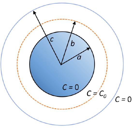Suppose a particle is released near a spherical absorber of radius a at a point \(r = b\). What is the probability that the particle will be absorbed at r = a rather than wandering off beyond an outer perimeter at \(r = c\)?

To solve this problem we solve for the steady-state flux at the surfaces a and c subject to the boundary conditions C(a) = 0, C(b) = C₀, and C(c) = 0. That is, the inner and outer surfaces are perfectly absorbing, but the concentration has a maximum value C(b) = C₀ at r = b.

We separate the problem into two zones, a-to-b and b-to-c, and apply the general solution eq. (10.3.3) to these zones with the appropriate boundary conditions to yield:

\[ \begin{aligned} &C(r) = \dfrac{C_0}{(1-a/b)} \left( 1-\dfrac{a}{r} \right) \qquad a \leq r \leq b \\ &C(r) = \dfrac{C_0}{(c/b-1)} \left( 1-\dfrac{a}{r} \right) \qquad b \leq r \leq c \end{aligned} \]

Then the radial flux density is:

\[ \begin{aligned} &J_r(r) = -\dfrac{DC_0}{(1-a/b)} \dfrac{a}{r^2} \qquad a\leq r \leq b \\ & J_r(r) = \dfrac{DC_0}{(c/b-1)} \dfrac{c}{r^2} \qquad \quad b \leq r \leq c \end{aligned} \]

Calculating the areas of the two absorbing surfaces and multiplying the flux densities by the areas gives the flux. The flux from the spherical shell source to the inner absorber is

\[ j_{in} = 4\pi DC_0 \dfrac{a}{(1-a/b)} \nonumber \]

and the flux from the spherical shell source to the outer absorber is

\[ j_{out} = 4\pi DC_0 \dfrac{c}{(c/b-1)} \nonumber \]

We obtain the probability that a particle released at r = b and absorbed at r = a from the ratio

\[ P_{capture} = \dfrac{j_{in}}{j_{in}+j_{out}}= \dfrac{a(c-b)}{b(c-a)} \nonumber \]

In the limit \(c \longrightarrow \infty \), this probability is just a/b. This is the probability of capture for the sphere of radius a immersed in an infinite medium. Note that this probability decreases only inversely with the radial distance b^–1, rather than the surface area of the sphere.

_________________________________

1. A. Walter and J. Gutknecht, Permeability of small nonelectrolytes through lipid bilayer membranes, J. Membr.Biol. 90, 207–217 (1986).

Readings

• H. C. Berg, Random Walks in Biology. (Princeton University Press, Princeton, N.J., 1993).
• K. Dill and S. Bromberg, Molecular Driving Forces: Statistical Thermodynamics in Biology, Chemistry, Physics, and Nanoscience. (Taylor & Francis Group, New York, 2010).