11.1: Random Walk and Diffusion

We want to describe the correspondence between a microscopic picture for the random walk of particles and macroscopic diffusion of particle concentration gradients. We will describe the statistics for the location of a random walker in one dimension (x), which is allowed to step a distance Δx to the right (+) or left (–) during each time interval Δt. At each time point a step must be taken left or right, and steps to left and right are equally probable.

Let’s begin by describing where the system is at after taking n steps qualitatively. We can relate the position of the system to where it was before taking a step by writing:

\[x(n) = x(n-1) \pm \Delta x \nonumber \]

This expression can be averaged over many steps:

\[ \begin{aligned} \langle x(n) \rangle &= \langle x(n-1) \pm \Delta x \rangle \\ &= \langle x(n-1) \rangle = \langle x(n-2) \rangle = ... = \langle x(0) \rangle \end{aligned} \]

Since there is equal probability of moving left or right with each step, the ±Δx term averages to zero, and \(\langle x \rangle\) does not change with time. The most probable position for any time will always be the starting point.

Now consider the variance in the displacement:

\[ \begin{aligned} \langle x^2(n)\rangle &= \langle x^2(n-1) \pm 2 \Delta x \, x(n-1)+(\Delta x )^2\rangle \\ &= \langle x^2(n-1) \rangle + (\Delta x)^2 \end{aligned} \]

In the first line, the middle term averages to zero, and the variance gains a factor of Δx². Repeating this process for each successive step back shows that the mean square displacement grows linearly in the number of steps.

\[ \begin{aligned} &\langle x^2(0) \rangle =0 \\ &\langle x^2(1) \rangle = (\delta x)^2 \\ &\langle x^2(2) \rangle = 2(\delta x )^2 \end{aligned} \]

\[ \vdots \nonumber \]

\[ \langle x^2 (n)\rangle = n(\Delta x)^2 \]

Qualitatively, these arguments indicate that the statistics of a random walker should have the same mean and variance as the concentration distribution for diffusion of particles from an initial position.

Random Walk Step Distribution Function

Now let’s look at this a little more carefully and describe the probability distribution for the position of particles after n steps, which we equate with the number of possible random walk trajectories that can lead to a particular displacement. What is the probability of starting at x₀ = 0 and reaching point x after n jumps separated by the time interval Δt?

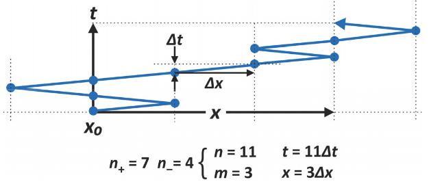
Similar to our discussion of the random walk polymer, we can express the displacement of a random jumper to the total number of jumps in the positive direction n₊ and in the negative direction n_–. If we make n total jumps, then

\[ n = n_++n_- \qquad \longrightarrow \qquad t=n \Delta t \nonumber \]

The total number of steps n is also our proxy for the length of time for a given trajectory, t. The distance between the initial and final position is related to the difference in + and ‒ steps:

\[ m = n_+-n_- \qquad \longrightarrow \qquad x=m\Delta x \nonumber \]

Here m is our proxy for the total displacement x. Note from these definitions we can express n₊ and n_– as

\[ n_{\pm} = \dfrac{n\pm m}{2} \]

The number of different ways of making n jumps with the constraint of n+ positive and n– negative jumps is

\[ \Omega = \dfrac{n!}{n_+!n_-!} \nonumber \]

The probability of observing a particular sequence of n “+” and “–” jumps is \( P(n) = (P_+)^{n_+} (P_-)^{n_-} = (1/2)^n\).

The total number of trajectories that are possible with n equally probably “+” and “‒” jumps is 2ⁿ, so the probability that any one sequence of n steps will end up at position m is given by Ω/2ⁿ or

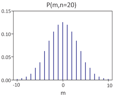
\[ \begin{aligned} P(m,n) &= \left( \dfrac{1}{2} \right)^n \dfrac{n!}{n_+!n_-!} \\ &= \left( \dfrac{1}{2} \right)^n \dfrac{n!}{\dfrac{n+m}{2}! \dfrac{n-m}{2}!} \end{aligned} \]

This is the binomial probability distribution function. Looking at the example below for twenty steps, we see \(\langle m\rangle =0\) and for a discrete probability distribution which has a Gaussian envelope.

For very large n, the distribution function becomes continuous. To see this, let’s apply Stirling’s approximation, \( n! \approx (n/e)^n \sqrt{2\pi n} \), and after a bit of manipulation we find¹

\[P(m,n) = \sqrt{\dfrac{2}{\pi n}} e^{-m^2/2n} \]

Note, this distribution has an envelope that follows a normal Gaussian distribution for a continuous variable where the variance σ² is proportional to the number of steps n.

To express this with a time variable, we instead insert n = t/Δt and m = x/Δx in eq. (11.1.3) to obtain the discrete probability distribution function:

\[ P(x,t) = \sqrt{\dfrac{\Delta t}{2\pi t}} \exp \left[ - \dfrac{\Delta t x^2}{2t(\Delta x)^2} \right] \nonumber \]

Note that we can re-write this discrete probability distribution similar to the continuum diffusion
solution

\[ P(x,t) = \sqrt{\dfrac{(\Delta x)^2}{4\pi Dt}}e^{-x^2/4Dt} \]

if we equate the variance and diffusion constant as

\[D = \dfrac{(\Delta x )^2}{2\Delta t} \nonumber \]

Equation (11.1.4) is slightly different because P is a unitless probability for finding the particle between x and x+Δx, rather than a continuous probability density ρ with units of m^-1: ρ(x,t) dx = P(x,t). Even so, eq. (11.1.4) suggests that the time-dependent probability distribution function for the random walk obeys a diffusion equation

\[ \dfrac{\partial P}{\partial t} = \Delta x D \dfrac{\partial^2 P}{\partial x^2} \qquad \qquad or \qquad \qquad \dfrac{\partial \rho}{\partial t} = D \dfrac{\partial^2 \rho}{\partial x^2} \]

Three‐Dimensional Random Walk

We can extend this treatment to diffusion from a point source in three dimensions, by using a random walk of n steps of length Δx on a 3D cubic lattice. The steps are divided into those taken in the x, y, and z directions:

\[ n = n_x+n_y+n_z \nonumber \]

and distance of the walker from the origin is obtained from the net displacement along the x, y, and z axes:

\[r = (x^2+y^2+z^2)^{1/2} = m\Delta x \\ m = \sqrt{m_x^2+m_y^2+m_z^2} \nonumber \]

For each time-interval the walker takes a step choosing the positive or negative direction along the x, y, and z axes with equal probability. Since each dimension is independent of the others

\[ P(r,n) = P(m_x,n_x)P(m_y,n_y)P(m_z,n_z) \nonumber \]

Looking at the radial displacement from the origin, we find

\[ \sigma_x^2 + \sigma_y^2 + \sigma_z^2 = \sigma_r^2 \nonumber \]

where

\[ \sigma_x^2 = \dfrac{(\Delta x )^2t}{\Delta t} \rightarrow 2D_xt \nonumber \]

but since each dimension is equally probable \(\sigma_r^2 = 3\sigma_x^2 \). Then using eq. (11.1.3)

\[ P(r,t) = \left( \dfrac{3\Delta x^2}{2\pi \sigma_r^2} \right)^{3/2} e^{-3r^2/2\sigma_r^2} \nonumber \]

where \(\sigma_r^2=6Dt\).

__________________________________________________

1. M. Daune, Molecular Biophysics: Structures in Motion. (Oxford University Press, New York, 1999), Ch. 7.