11.2: Markov Chain and Stochastic Processes

Working again with the same problem in one dimension, let’s try and write an equation of motion for the random walk probability distribution: \(P(x,t)\).

• This is an example of a stochastic process, in which the evolution of a system in time and space has a random variable that needs to be treated statistically.
• As above, the movement of a walker only depends on the position where it is at, and not on any preceding steps. When the system has no memory of where it was earlier, we call it a Markovian system.
• Generally speaking, there are many flavors of a stochastic problem in which you describe the probability of being at a position \(x\) at time \(t\), and these can be categorized by whether \(x\) and \(t\) are treated as continuous or discrete variables. The class of problem we are discussing with discrete \(x\) and \(t\) points is known as a Markov Chain. The case where space is treated discretely and time continuously results in a Master Equation, whereas a Langevin equation or Fokker–Planck equation describes the case of continuous \(x\) and \(t\).
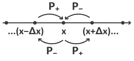
• To describe the walkers time-dependence, we relate the probability distribution at one point in time, \(P(x,t+Δt)\), to the probability distribution for the preceding time step, \(P(x,t)\) in terms of the probabilities of a walker making a step to the right (\(P_+\)) or to the left (\(P_-\)) during the interval \(Δt\). Note, when \(P_+\neq P_-\), there is a stepping bias in the system. If \(P_+ + P_-<1\), there is a resistance to stepping either as a result of an energy barrier or excluded volume on the chain.
• In addition to the loss of probability by stepping away from x to the left or right, we need to account for the steps from adjacent sites that end at \(x\).

Then the probability of observing the particle at position \(x\) during the interval \(Δ\)t is:

\[\begin{aligned} P(x,t+\Delta t) &= P(x,t)-P_+\cdot P(x,t) -P_- \cdot P(x,t) +P_+\cdot P(x-\Delta x,t)+P_- \cdot P(x+\Delta x,t) \\[4pt] &= (1-P_+-P_-) \cdot P(x,t)+P_+ \cdot P(x-\Delta x,t) +P_- \cdot P(x+\Delta x,t) \\[4pt] &= P(x,t) + P_+[P(x-\Delta x,t)-P(x,t)]+ P_-[P(x+\Delta x,t)-P(x,t)] \end{aligned} \]

and the net change probability is

\[ P(x,t+\Delta t) - P(x,t) = P_+[P(x-\Delta x,t) - P(x,t)]+P_-[P(x+\Delta x,t)-P(x,t)] \nonumber \]

We can cast this as a time-derivative if we divide the change of probability by the time-step Δt:

\[ \begin{aligned} \dfrac{\partial P}{\partial t} &= \dfrac{P(x,t+\Delta t)-P(x,t)}{\Delta t} \\[4pt] &= P_+[P(x-\Delta x,t) - P(x,t)]+P_-[P(x+\Delta x,t)-P(x,t)] \\[4pt] &= P_+ \Delta P_-(x,t)+P_-\Delta P_+(x,t) \end{aligned} \] \[\]

Where \(P_{\pm} = P_{\pm} / \Delta t\) is the right and left stepping rate, and \( \Delta P_{\pm}(x,t) = P(x \pm \Delta x,t)-P(x,t) \)

We would like to show that this random walk model results in a diffusion equation for the probability density ρ(x,t) we deduced in Equation (11.1.5). To simplify, we assume that the left and right stepping probabilities \(P_+=P_-=\frac{1}{2}\), and substitute

\[ P(x,t) = \rho (x,t) dx \nonumber \]

into Equation (11.2.1):

\[ \dfrac{\partial \rho}{\partial t} = P[\rho(x-\Delta x,t)-2 \rho (x,t)+\rho (x+\Delta x,t)] \nonumber \]

where \(P=1/2 \, \Delta t \). We then expand these probability density terms in x as

\[ \rho (x,t) = \rho (0,t) + \dfrac{\partial \rho}{\partial x} x+\dfrac{1}{2} \dfrac{\partial^2 \rho}{\partial x^2} x^2 \nonumber \]

and find that the probability density follows a diffusion equation

\[ \dfrac{\partial \rho}{\partial t} = D \dfrac{\partial^2 \rho}{\partial x^2} \nonumber \]

where \(D= \Delta x^2/2 \Delta t\).

___________________________________

Reading Materials

• A. Nitzan, Chemical Dynamics in Condensed Phases: Relaxation, Transfer and Reactions in Condensed Molecular Systems. (Oxford University Press, New York, 2006).