14.1: Sampling and Statistical Analysis of Data

Learning Objectives:

• Describe and explain the importance of the concept of “sampling” in analytical methods of analysis.
• Describe and discuss the sources and types of sampling error and uncer- tainty in measurement.
• Acquire the techniques for handling numbers associated with measure-ments: scientific notation and significant figures.
• Explain the concept of data rejection (or elimination) and comparison of measurements.
• Apply simple statistics and error analysis to determine the reliability of analytical chemical measurements and data.

This activity comprises two fairly distinct study topics: Sampling and Statistical analysis of data. Under “Sampling”, you will be introduced to the concept and challenges of sampling as a means to acquiring a representative laboratory sam- ple from the original bulk specimen. At the end of the subtopic on “sampling”, you will not only appreciate that a sampling method adopted by an analyst is an integral part of any analytical methods, but will also discover that it is usually the most challenging part of an analysis process. Another very important stage in any analytical method of analysis is evaluation of results, where statistical tests (i.e., quantities that describe a distribution of, say, experimentally measureddata) are always carried out to determine confidence in our acquired data. In thelatter part of this activity, you will be introduced to the challenges encountered by an analytical chemist when determining the uncertainity associated with every measurement during a chemical analysis process, in a bid to determine the most probable result. You will be introduced to ways of describing and reducing, if necessary, this uncertainity in measurements through statistical techniques.

Key Concepts

• Accuracy: refers to how closely the measured value of a quantity corresponds to its “true” value.
• Determinate errors: these are mistakes, which are often referred to as “bias”. In theory, these could be eliminated by careful technique.
• Error analysis: study of uncertainties in physical measurements.
• Indeterminate errors: these are errors caused by the need to make estimates inthe last figure of a measurement, by noise present in instruments, etc. Such errorscan be reduced, but never entirely eliminated.
• Mean (m): defined mathematically as the sum of the values, divided by thenumber of measurements.
• Median: is the central point in a data set. Half of all the values in a set will lie above the median, half will lie below the median. If the set contains an odd number of datum points, the median will be the central point of that set. If the set contains an even number of points, the median will be the average of the two central points. In populations where errors are evenly distributed about the mean, the mean and median will have the same value.
• Precision: expresses the degree of reproducibility, or agreement between repeated measurements.
• Range: is sometimes referred to as the spread and is simply the difference between the largest and the smallest values in a data set.
• Random Error: error that varies from one measurement to another in an unpre- dictable manner in a set of measurements.
• Sample: a substance or portion of a substance about which analytical information is sought.
• Sampling: operations involved in procuring a reasonable amount of material that is representative of the whole bulk specimen. This is usually the most challenging part of chemical analysis.
• Sampling error: error due to sampling process(es).
• Significant figures: the minimum number of digits that one can use to represent a value without loss of accuracy. It is basically the number of digits that one is certain about.
• Standard deviation (s): this is one measure of how closely the individual results or measurements agree with each other. It is a statistically useful description of the scatter of the values determined in a series of runs.
• Variance (s²): this is simply the square of the standard deviation. It is another method of describing precision and is often referred to as the coefficientof variation.

Introduction to the activity

A typical analytical method of analysis comprises seven important stages, namely;plan of analysis (involves determination of sample to be analysed, analyte, and level of accuracy needed); sampling; sample preparation (involves sample disso- lution, workup, reaction, etc); isolation of analyte (e.g., separation, purification,etc); measurement of analyte; standardization of method (instrumental methods need to be standardized inorder to get reliable results); and evaluation of results (statistical tests to establish most probable data). Of these stages, sampling is often the most challenging for any analytical chemist: the ability to acquire a laboratory sample that is representative of the bulk specimen for analysis. The- refore, sampling is an integral and a significant part of any chemical analysisand requires special attention. Furthermore, we know that analytical work in general, results in the generation of numerical data and that operations such as weighing, diluting, etc, are common to almost every analytical procedure. The results of such operations, together with instrumental outputs, are often combi- ned mathematically to obtain a result or a series of results. How these resultsare reported is important in determining their significance. It is important that analytical results be reported in a clear, unbiased manner that is truly reflectiveof the very operations that go into the result. Data need to be reported with theproper number of significant digits and rounded off correctly. In short, at the endof, say a chemical analysis procedure, the analyst is often confronted with theissue of reliability of the measurement or data acquired, hence the significanceof the stage of evaluation of results, where statistical tests are done to determineconfidence limits in acquired data.

In this present activity, procedures and the quantities that describe a distribution of data will be covered and the sources of possible error in experimental measu- rements will be explored.

Sampling errors

Biased or nonrepresentative sampling and contamination of samples during orafter their collection are two sources of sampling error that can lead to significanterrors. Now, while selecting an appropriate method helps ensure that an analysis is accurate, it does not guarantee, however, that the result of the analysis willbe sufficient to solve the problem under investigation or that a proposed answerwill be correct. These latter concerns are addressed by carefully collecting the samples to be analyzed. Hence the import of studying “proper sampling strate-gies”. It is important to note that the final result in the determination of say, thecopper content in an ore sample would typically be a number(s) which indicates the concentration(s) of a compound(s) in the sample.

Uncertainty in measurements

However, there is always some uncertainity associated with each operation or measurement in an analysis and thus there is always some uncertainity in thefinal result. Knowing the uncertainty is as important as knowning the final result.Having data that are so uncertain as to be useless is no better than having no data at all. Thus, there is a need to determine some way of describing and reducing, if necessary, this uncertainty. Hence the importance of the study of the subtopic ofStatistics, which assists us in determining the most probable result and provides us the quantities that best describe a distribution of data. This subtopic of Staisticswill form a significant part of this learning activity.

List of other compulsory readings

Material and Matters (Reading #3)
Measurements and significant figures (Reading #4) Units and dimensions (Reading #5)
Significant figures (Reading #6)
Significant figures and rounding off (Reading #7) Measurements (Reading #8)

List of relevant resources

List of relevant useful links

www.chem1.com/acad/webtext/matmeasure/mm1.html

Deals with Units of measurements.

www.chem1.com/acad/webtext/matmeasure/mm2.html

Deals with measurement error.

www.chem1.com/acad/webtext/matmeasure/mm3.html

Deals with significant figures.

www.chem1.com/acad/webtext/matmeasure/mm4.html

Deals with testing reliability of data or measurements.

www.chem1.com/acad/webtext/matmeasure/mm5.html

Covers useful material on simple statistics.

Detailed description of the actvity

Studying a problem through the use of statistical data analysis often involves fourbasic steps, namely; (a) defining the problem, (b) collecting the data (c) analyzingthe data, and (d) reporting the results. In order to obtain accurate data about aproblem, an exact definition of the problem must be made. Otherwise, it would be extremely difficult to gather data without a clear definition of the problem. On collection of data, one must start with an emphasis on the importance of defi- ning the population, the set of all elements of interest in a study, about which we seek to make inferences. Here, all the requirements of sampling, the operations involved in getting a reasonableamount of material that is representative of the whole population, and experimental design must be met. Sampling is usually themost difficult step in the entire analytical process of chemical analysis, particu- larly where large quantities of samples (a sample is the subset of the population) to be analysed are concerned. Proper sampling methods should ensure that the sample obtained for analysis is representative of the material to be analyzed and that the sample that is analyzed in the laboratory is homogeneous. The more representative and homogeneous the samples are, the smaller will be the part of the analysis error that is due to the sampling step. Note that, an analysis cannot be more precise than the least precise operation.

The main idea of statistical inference is to take a random finite sample from apopulation (since it is not practically feasible to test the entire population) and then use the information from the sample to make inferences about particular population characteristics or attributes such as mean (measure of central ten- dency), the standard deviation (measure of spread), or the proportion of items in the population that have a certain characteristic. A sample is therefore the only realistic way to obtain data due to the time and cost contraints. It also saves effort. Furthermore, a sample can, in some cases, provide as much or more accuracy than a corresponding study that would otherwise attempt to investigate the entire population (careful collection of data from a sample will often provide better information than a less careful study that attempts to look at everything). Note that data can be either qualitative, labels or names used to identify an attribute of each element of the population, or quantitative, numeric values that indicate how much or how many a particular element exists in the entire population.

Statistical analysis of data: Assessing the reliability of measurements through simple statistics

In these modern times, the public is continuously bombarded with data on all sorts of information. These come in various forms such as public opinion polls, government information, and even statements from politicians. Quite often, the public is wonders about the “truth” or reliability of such information, particularly in instances where numbers are given. Much of such information often takes advantage of the average person’s inability to make informed judgement on the reliability of the data or information being given.

In science however, data is collected and measurements are made in order to get closer to the “truth” being sought. The reliability of such data or measurements must then be quantitatively assessed before disseminating the information to the stakeholders. Typical activities in a chemistry laboratory involve measurement of quantities that can assume a continuous range of values (e.g. Masses, volumes, etc). These measurements consist of two parts: the reported value itself (never an exactly known number) and the uncertainty associated with the measurement. All such measurements are subject to error which contributes to the uncertainty of the result. Our main concern here is with the kinds of errors that are inherent in any act of measuring (not outright mistakes such as incorrect use of an instru- ment or failure to read a scale properly; although such gross errors do sometimes occur and could yield quite unexpected results).

Experimental Error and Data Analysis

Theory:

Any measurement of a physical quantity always involves some uncertainty or experimental error. This means that if we measure some quantity and then repeat the measurement, we will most certainly obtain a different value the second time around. The question then is: Is it possible to know the true value of a physical quantity? The answer to this question is that we cannot. However, with grea- ter care during measurements and with the application of more experimentalmethods, we can reduce the errors and, thereby gain better confidence that themeasurements are closer to the true value. Thus, one should not only report a result of a measurement but also give some indication of the uncertainty of the experimental data.

Experimental error measured by its accuracy and precision, is defined as thedifference between a measurement and the true value or the difference between two measured values. These two terms have often been used synonymously, but in experimental measurements there is an important distinction between them.

Accuracy measures how close the measured value is to the true value or accepted value. In other words, how correct the measurement is. Quite often however, the true or accepted value of a physical quantity may not be known, in which case it is sometimes impossible to determine the accuracy of a measurement.

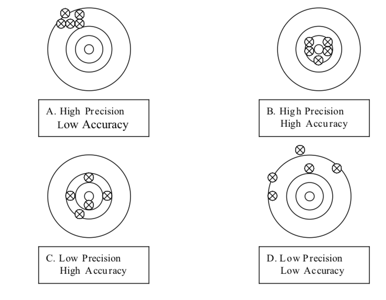
Precision refers to the degree of agreement among repeated measurements or how closely two or more measurements agree with each other. The term is so- metimes referred to as repeatability or reproducibility. Infact, a measurement that is highly reproducible tends to give values which are very close to each other. The concepts of precision and accuracy are demonstrated by the series oftargets shown in the figure below. If the centre of the target is the “true value”,then A is very precise (reproducible) but not accurate; target B demonstrates both precision and accuracy (and this is the goal in a laboratory); average of target C’s scores give an accurate result but the precision is poor; and target D is neithet precise nor accurate.

It is important to note that no matter how keenly planned and executed, all experiments have some degree of error or uncertainty. Thus, one should learn how to identify, correct, or evaluate sources of error in an experiment and how to express the accuracy and precision of measurements when collecting data or reporting results.

Types of experimental errors

Three general types of errors are encountered in a typical laboratory experiment measurements: random or statistical errors, systematic errors, and gross errors.

Random (or indeterminate) errors arises due to some uncontrollable fluctuations in variables that affect experimental measurements and therefore has no specific cause. These errors cannot be positively identified and do not have a definite measurable value; instead, they fluctuate in a random manner. These errors af- fect the precision of a measurement and are sometimes referred to as two-sided errors because in the absence of other types of errors, repeated measurementsyield results that fluctuate above and below the true value. With sufficientlylarge number of experimental measurements, an evenly distributed data scattered around an average value or mean is achieved. Thus, precision of measurements subject to random errors can be improved by repeated measurements. Random errors can be easily detected and can be reduced by repeating the measurementor by refining the measurement method or technique.

Systematic (or determinate) errors are instrumental, methodology-based, or individual mistakes that lead to “skewed” data, that is consistently deviated in one direction from the true value. These type of errors arises due to somespecific cause and does not lead to scattering of results around the actual value. Systematic errors can be identified and eliminated with careful inspection of theexperimental methods, or cross-calibration of instruments.

A determinate error can be further categorized into two: constant determinate error and proportional determinate error.

Constant determinate error (e_cd) gives the same amount of error independent of the concentration of the substance being analyzed, whereas proportional determinate error (e_pd) depends directly on the concentration of the substance being analyzed (i.e., e_pd = K C), where K is a constant and C is the concentration of the analyte.

Therefore, the total determinate error (E_td) will be the sum of the proportional and constant determinate errors, i.e.,

$$\bf{E}_{td}=\bf{e}_{cd}+\bf{e}_{pd}$$

Gross errors are caused by an experimenter’s carelessness or equipment failure. As a result, one gets measurements, outliers, that are quite different from the other sets of similar measurements (i.e., the outliers are so far above or below the true value that they are usually discarded when assessing data. The “Q-test” (discussed later) is a systematic way to determine if a data point should be dis- carded or not.

Example:

Classify each of the following as determinate or random error:

1. Error arising due to the incomplete precipitation of an analyte in a gravi- metric analysis.
2. Error arising due to delayed colour formation by an indicator in an acid- base titration.

Solution:

1. Incomplete precipitation of an analyte in gravimetric analysis results in a determinate error. The mass of the precipitate will be consistently less than the actual mass of the precipitate.
2. Delayed color formation by an indicator in an acid-base titration also introduces a determinate error. Since excess titrant is added after the equivalence point, the calculated concentration of the titrand will be consistently higher than the value obtained by using an indicator which changes color exactly at the equivalence point is used.

Exercise 1:

An analyst determines the concentration of potassium in five replicatesof a standard water sample with an accepted value for its potassium concentration of 15 ppm by Flame Atomic Emission Spectrophotometry technique. The resultshe obtained in each of the five analyses in ppm were: 14.8, 15.12, 15.31, 14.95and 15.03. Classify the error in the analysis described above for the determination of potassium in the standard water sample as determinate or random.

Exercise 2:

Classify each of the errors described below as ‘constant determinate error’ or ‘proportional determinate error

1. The error introduced when a balance that is not calibrated is used for weighing samples?
2. The error introduced when preparing the same volumes of solutions magnesium ions having different concentrations from a MgCl₂ salt that contains 0.5 g Ca²⁺ impurity per 1.0 mol (95 g) of MgCl₂?

Expressing and Calculating Experimental Error and Uncertainty

An analyst reporting results of an experiment is often required to include accuracy and precision of the experimental measurements in the report to provide some credence to the data. There are various ways of describing the degree of accuracy or presision of data and the common ways are provided below, with examples or illustrations.

Significant Figures: Except in situations where numbers or quantities under in- vestigation are integers (for example counting the number of boys in a class) it is often impossible to get or obtain the exact value of the quantity under investigation. It is precisely for this reason that it is important to indicate the margin of error in a measurement by clearly indicating the number of significant figures, which arereally the meanigful digits in a measurement or calculated quantity.

When significant figures are used usually the last is understood to be uncertain.

For example, the average of the experimental values 51.60, 51.46, 51.55, and 51.61 is 51.555. The corresponding standard deviation of the sum is ± 0.069. It is clear from the above that the number in the second decimal place of the experimental values is subject to uncertainty. This implies that all the numbers in succeeding decimal places are without meaning, and we are therefore forced to round the average value accordingly. We must however, consider the question of taking 51.55 or 51.56, given that 51.555 is equally spaced between them. As a guide, when rounding a 5, always round to the nearest even number so that any tendency to round in a set direction is eliminated, since there is an equal likelihood that the nearest even number will be the higher or the lower in any given situation. Thus, we can report the above results as 51.56 ± 0.07.

It is the most general way to show “how well” a number or measurement isknown. The proper usage of significant figures becomes even more importantin today’s world, where spreadsheets, hand-held calculators, and instrumental digital readout systems are capable of generating numbers to almost any degree of apparent precision, which may be much different than the actual precision associated with a measurement.

Illustration:

A measurement of volume using a graduated measuring cylinder with 1-mL graduation markings will be reported with a precision of ± 0.1 mL, while a measurement of length using a meter-rule with 1-mm graduations will be reported with a precision of ± 0.1 mm. The treatment for digital instruments is however different owing to their increased level of accuracy. Infact, most manufacturers report precision of measurements made by digital instruments with a precision of± 1/2 of the smallest unit measurable by the instrument. For instance, a digital multimeter reads 1.384 volts; the precision of the multimeter measurement is ±1/2 of 0.001 volts or ± 0.0005 volts. Thus, the significant numbers depend on the quality of the instrument and the fineness of its measuring scale.

To express results with the correct number of significant figures or digits, a few simple rules exist that will ensure that the final result should never contain any more significant figures than the least precise data used to calculate it.

• All non-zero digits are significant. Thus 789 km has three significant figures; 1.234kg has four significant figs and so on
• Zeros between non-zero digits are significant. Thus 101 years contains three significant figures, 10,501m contains five significant figures and soon.
• The most significant digit in a reported result is the left-most non-zero digit: 359.742 (3 is the most significant digit). (How does this help to determine the number of significant figures in a measurement? I wouldrather include this:
• Zeros to the left of the first non-zero digit are not significant. Their purposeis to indicate the placement of the decimal point. For examplle, 0.008Lcontains one significant figure, 0.000423g contains three significant figuresand so on.
• If a number is greater than 1 then all the zeros to the right of the decimalpoint count as significant figures. Thus 22.0mg has three significant figures; 40.065 has five significant figures. If a number is less than1, then onlythe zeros that are at the end of the number and the zeros that are betweennonzero digits are significant. For example, 0.090 g has two significant figures, 0.1006 m has four significant figures, and so on.
• For numbers without decimal points, the trailing zeros (i.e. zeros afterthe last nonzero digit) may or may not be significant. Thus 500cm may have one significant figure (the digit 5), two significant figures (50) or three significant figures (500). It is not possible to know hich is correct without more information. By using scientific notation we avoid suchambiguity. We can therefore express the number 400 as 4 x 102 for onesignificant figure or 4.00 x 10-2 for three significant figures.
• If there is a decimal point, the least significant digit in a reported result is the right-most digit (whether zero or not): 359.742 (2 is the least significantdigit). If there is no decimal point present, the right-most non-zero digitis the least significant digit.
• The number of digits between and including the most and least significant digit is the number of significant digits in the result: 359.742 (there are six significant digits).

Exercise 1:

Determine the number of significant figures in the following measu- rements: (a) 478m (b) 12.01g (c) 0.043kg (d) 7000mL (e) 6.023 x 10²³

Note that, the proper number of digits used to express the result of an arithmetic operation (such as addition, subtraction, multiplication, and division) can be obtained by remembering the principle stated above: that numerical results are reported with a precision near that of the least precise numerical measurement used to generate the number.

Illustration:

For Addition and subtraction

The general guideline when adding or subtracting numerical values is that the answer should have decimal places equal to that of the component with the least number of decimal places. Thus, 21.1 + 2.037 + 6.13 = 29.267 = 29.3, since component 21.1 has the least number of decimal places.

For Multiplication and Division

The general guideline is that the answer has the same number of significant figures as the number with the fewest significant figures: Thus

\[{56 \times 0.003462\times 43.72\over1.684}=4.975740998 \approx 5.0\]

since one of the measurements (i.e., 56) has only two significant figures.

Exercise 1:

To how many significant figures ought the result of the sum of thevalues 3.2, 0.030, and 6.31 be reported and what is the calculated uncertainty?

Exercise 2:

To how many significant figures ought the result of the operation (28.5 x 27) / 352.3 be reported and what is the calculated uncertainty?

Percent Error (% Error): This is sometimes referred to as fractional difference, and measures the accuracy of a measurement by the difference between a measured value or experimental value E and a true or accepted value A. Therefore

\[\% Error = ({|E-A|\over A})\ x \ 100\%\]

Percent Difference (% Difference): This measures precision of two measure- ments by the difference between the measured experimental values E1 and E2expressed as a fraction of the average of the two values. Thus

\[\%Difference={({|E1-E2|\over{E1+E2\over2}})\ x\ 100\%}\]

Mean and Standard Deviation

Ordinarily, a single measurement of a quantity is not considered scientifically sufficient to convey any meaningful information about the quality of the measu- rement. One may need to take repeated measurements to establish how consistent the measurements are. When a measurement is repeated several times, we often see the measured values grouped or scattered around some central value. This grouping can be described with two numbers: a single representative number called the mean, which measures the central value, and the standard deviation, which describes the spread or deviation of the measured values about the mean.

The mean ( x̄ ) is the sum of the individual measurements (xi) of some quantity divided by the number of measurements (N). The mean is calculated by the formula:

\[\bar{x}={1\over N}\sum_{i=1}^n\bf{x}_i={1\over N}(\bf{x}_1+\bf{x}_2+\bf{x}_3+...+\bf{x}_{N-1}+\bf{x}_N)\]

where x̄ is the i^th measured value of x.

The standard deviation of the measured values, represented by the symbol, σ_x is determined using the formula:

\[\bf{\sigma}_x=\sqrt{{1\over{N-1}}\sum_{i=1}^N(\bf{x}_i-\bar{x})}\]

The standard deviation is sometimes referred to as the mean square deviation. Note that, the larger the standard deviation, the more widely spread that data is about the mean.

The simplest and most frequently asked question is: “What is the typical value that best represents experimental measurements, and how reliable is it?”

Consider a set of N (=7) measurements of a given property (e.g., mass) arran- ged in increasing order (i.e., x1, x2, x3, x4, x5, x6 and x7). Several useful anduncomplicated methods are available for finding the most probable value and its confidence interval, and for comparing such results as seen above. However,when the number of measurements available N are few, the median is often more appropriate than the mean. In addition to the standard deviation, the range is also used to describe the scatter in a set of measurements or observations. The range is simply the difference between the largest and the smallest values or observations in a data set. Range = x_max – x_min, where x_max and x_min are the largest and smallest observations in a data set, respectively.

The median is defined as the value that bisects the set of N ordered observations, i.e., it is the central point in an ordered data set. If the N is odd, then (N-1)/2 measurements are smaller than the median, and the next higher value is reported as the median (i.e., the median is the central point of that set). In our illustra- tion above, the 4th measurement (i.e., x4) would be the median. If the data set contains an even number of points, the median will be the average of the two central points. If, however, the data set contains an even number of points, themedian will be the average of the two central points.

Example 1:For N = 6 and x() = 2, 3, 3, 5, 6, 7; median = (3+5)/2 = 4; the mean= (2 + 3 + 3 + 5 + 6 + 7)/6 = 4.33; and the range = (7 – 2) = 5.

Note: The median can thus serve as a check on the calculated mean. In samples where errors are evenly distributed about the mean, the mean and median will have the same value. Often relative standard deviation is more useful in a prac- tical sense than the standard deviation as it immediately gives one an idea of the level of precision of the data set relative to its individual values.

Relative standard deviation (rel. std. dev.) is defined as the ratio of the standarddeviation to the mean. The formula for it evaluation is:

\[rel.std.dev.={\bf{\sigma}\over\bar{x}}\]

Example 2. Assume that the following values were obtained in the analysis of the weight of iron in 2.0000g portions of an ore sample: 0.3791, 0.3784, 0.3793, 0.3779, and 0.3797 g.

xi (g)	(xi-x̄)^2 (g)^2
0.3791	(0.3791 - 0.37888)^2= 4.84 x 10^-8
0.3784	(0.3784 – 0.37888)^2= 2.30 x 10^-7
0.3793	(0.3793 – 0.37888)^2 = 1.76 x 10^-7
0.3779	(0.3779 – 0.37888)^2 = 9.60 x 10^-7
0.3797	(0.3797 – 0.37888)^2 = 6.72 x 10^-7
∑xi = 1.8944	∑(xi - x̄)^2 = 2.09 x 10^-6

The mean = x̄ = 1.8944g / 5 = 0.37888g

The standard deviation = σ_x = 2.09 x 10^-6 g²)/4 = 5.2 x 10^-7 g²

Rel. std. dev. = sr = 0.00072g/0.37888g = 0.0019

% Rel. std. dev. = (0.0019) x 100 = 0.19%

To easily see the range and median it is convenient to arrange the data in terms of increasing or decreasing values. Thus: 0.3779, 0.3784, 0.3791, 0.3793, and 0.3797 g. Since this data set has an odd number of trials, the median is simply the middle datum or 3^rd datum, 0.3791 g. Note that for a finite data set the median andmean are not necessarily identical. The range is 0.3797 – 0.3779 g or 0.0018.

Example 3. The concentration of arsenic in a standard reference material which contains 2.35 mg/L arsenic was determined in a laboratory by four students (St1, St2, St3, and St4) who carried out replicate analyses. The experimental values as determined and reported by each of student are listed in the table below. Classify the set of results given by the students as: accurate; precise; accurate and precise; and neither accurate nor precise.

Trial No	Concentration of Arsenic (in mg/L)
	St1	St2	St3	St4
1	2.35	2.54	2.25	2.45
2	2.32	2.52	2.52	2.22
3	2.36	2.51	2.10	2.65
4	2.34	2.52	2.58	2.34
5	2.30	2.53	2.54	2.78
6	2.35	2.52	2.01	2.58
Mean	2.34	2.52	2.33	2.50

Solution

• The set of results as obtained by St1 and St2 (see columns 1 and 2) are close to each other. However, the calculated mean value of the six trials (the value reported as the most probable value of arsenic concentration in the reference material) as reported by St1 is close to the reported true value of 2.35 mg/L while that of St2 is relatively far from this true value. It can then be concluded that the analytical result reported by St1 is both precise and accurate while that for St2 is precise but not accurate.
• The set of values from the six trials by students St3 and St4 appear re- latively far apart from each other. However, the mean of the analytical results reported by St3 is closer to the true value while that of St4 is not. It can therefore be concluded that the analytical result reported by St3 isaccurate but not precise; while that for St4 is neither precise nor accurate.

Reporting the Results of an Experimental Measurement

Results of an experimental measurement by an analyst should always comprise of two parts: The first, is the best estimate of the measurement which is usually reported as the mean of the measurements. The second, is the variation of the measurements, which is usually reported as the standard deviation, of the measurements. The measured quantity will then be known to have a best estimate equal to the average of the experimental values, and that it lies between ( x̄+σ_x) and ( x̄-σ_x). Thus, any experimental measurement should always then be reported in the form:

\[x=\bar{x}\pm\bf{\sigma}_x\]

Example 3:Consider the table below which contains 30 measurements of the mass, m of a sample of some unknown material.

Table showing measured mass in kg of an unknown sample material

1.09 1.14 1.06

1.01 1.03 1.12

1.10 1.17 1.00

1.14 1.09 1.10

1.16 1.09 1.07

1.11 1.15 1.08

1.04 1.06 1.07

1.11 1.15 1.08

1.04 1.06 1.07

1.16 1.12 1.14

1.13 1.08 1.11

1.17 1.20 1.05

For the 30 measurements, the mean mass (in kg) =1/30(33.04 kg)=1.10 kg

The standard deviation =

\[\bf{\sigma}_x=\sqrt{1\over{N-1}\sum_{i=1}^N(\bf{x}_i-\bar{x})^2}=\sqrt{1\over{30-1}\sum_{i=1}^{30}(\bf{x}_i-\bar{1.10\ kg})^2}=0.05\ kg\]

The measured mass of the unknown sample is then reported as = 1.10 ± 0.05kg

Statistical Tests

Sometimes a value in a data set appears so far removed from the rest of the values that one suspects that that value (called an outlier) must have been the result of some unknown large error not present in any of the other trials. Statisticians have devised many rejection tests for the detection of non-random errors. We will consider only one of the tests developed to determine whether an outlier could be rejected on statistical rather than arbitrary grounds and it is the Q test. Its details are presented below.

The Q test: Rejecting data.

Note that we can always reject a data point if something is known to be “wrong” with with the data or we may be able to reject outliers if they pass a statistical test that suggests that the probability of getting such a high (or low) value by chance is so slight that there is probably an error in the measurement and that it can be discarded. The statistical test is through the Q test outline below.

The Q test is a very simple test for the rejection of outliers. In this test one calculates a number called Q_exp and compares it with values, termed Q_crit, from a table. If Q_exp > Q_crit, then the number can be rejected on statistical grounds. Q_exp is calculated as follows:

\[\bf{Q}_{exp}={|questionable\ value\ -\ its \ nearest\ neighbour|\over range}\]

An example will illustrate the use of this test.
Example 4. Suppose that the following data are available: 25.27, 25.32, 25.34, and 25.61. It looks like the largest datum is suspect. Q_exp is then calculated.

Q_exp = (25.61 – 25.34)/(25.61-25.27) = 0.79

The values of Q_crit are then examined in statistical tables. These values depend on the number of trials in the data set, in this case 4. For example, the table below shows the values of Q for rejection of data at the 90% confidence level.

Table 4-4 Critical Values for the Rejection Quotient Q*
	Qcrit (Reject if Qexp>Qcrit)
Number of Observations	90% confidence	95% confidence	99% confidence
3	0.941	0.970	0.994
4	0.765	0.829	0.926
5	0.642	0.710	0.821
6	0.560	0.625	0.740
7	0.507	0.568	0.680
8	0.468	0.526	0.634
9	0.437	0.493	0.598
10	0.412	0.466	0.568

From: Skoog, West, Holle, ""Intro to analytical Chemistry. 7^th Ed. Thomson Publishing

The values are as follows:

Q_crit = 0.76 at 90% confidence

Q_crit = 0.85 at 96% confidence

Q_crit = 0.93 at 99% confidence

Since Q_exp > Q_crit at 90% confidence, the value of 25.61 can be rejected with 90% confidence.

What does this mean? It means that in rejecting the datum the experimentalist will be right an average of 9 times out of 10, or that the chances of the point actually being bad are 90%.

Is this the one time out of 10 that the point is good? This is not known! When data are rejected, there is always a risk of rejecting a good point and biasing the results in the process. Since Q_exp < Q_crit at the 96% and 99% levels, the datum cannot be rejected at these levels. What this says is that if one wants to be right 96 times or more out of 100, one cannot reject the datum. It is up to you to selectthe level of confidence you wish to use.

Exercise 1: Figure 1 below shows several separate steps involved in a typical total chemical analysis process in a chemical laboratory. Each step of the chemical analysis process has some random error associated with it. It is therefore clear that if a major error is made in any single step of the analysis it is unlikely that the result of the analysis can be correct even if the remaining steps are performed with little error. Discuss and list the possible sources of error an analyst is likelyto commit in each of the analytical steps given in figure 1, when determining the concentration of iron in a soil sample spectrophotometrically.

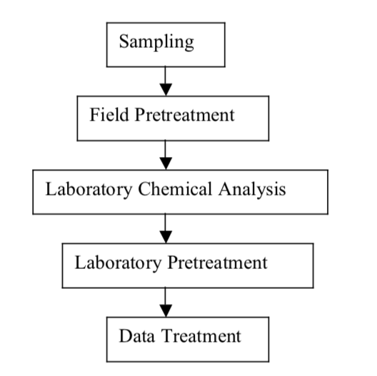
Figure 1. Block diagram of the major steps in a typical total chemical analysis process

Exercise 2:

In groups of atleast 2 people, obtain twenty-10 cent coins and de- termine the weight of each coin separately. Calculate the median, mean, range, standard deviation, relative standard deviation, % relative standard deviation and variance of your measurements

Exercise 3:

Calculate the σ and s (a) for each of the first 3, 10, 15 & 20 measu- rements you carried out in Exercise 2 to determine the mass of a 10 cents coin. b) compare the difference between the σ and s values you obtained in each case and describe your observation on the difference between the two values as the number of replicate analysis increase.

Exercise 4 :

Using data obtained in Exercise 2, determine the percent of your results that fall within the range of one, two, and three standard deviations, i.e., the results within μ± σ, μ± 2σ, μ± 3σ. Based on your findings, can you concludethat the results you obtained in determining the mass of a 10 cents coin (Exercise 2) yield a normal distribution curve?

Exercise 5 :

​​​​​​​​​​​​​​Refer to your results of Exercise 3 and (a) calculate the RSD and % RSD for the 3, 10, 15 and 20 measurements (b) compare the values you obtained and give a conclusion on what happens to the RSD and %RSD values as the number of replicate analyses increase.

Exercise 6:

(a) Calculate the variances for the values you obtained in the measurements i)1–5, ii)6–10, iii)11–15, iv) 16–20, and v)1–20, inactivity 1.

(b) Add the values you found in i, ii, iii, iv and compare the sum with the value you obtained in v.

(c) Calculate the standard deviations for the measurements given in i, ii, iii, iv and v of question a.

(d) Repeat what you did in question ‘b’ for standard deviation

(e) Based on your findings, give conclusions on the additiveness or non-ad- ditiveness of variance and standard deviation.

​​​​​​​ ​​​​​​​Problem 7: Compute the mean, median, range, absolute and relative standard deviations for the following set of numbers: 73.8, 73.5, 74.2, 74.1, 73.6, and 73.5.

Problem 8: Calculate the mean and relative standard deviation in ppt of the following data set: 41.29, 41.31, 41.30, 41.29, 41.35, 41.30, 41.28.

Problem 9: A group of students is asked to read a buret and produces the following data set: 31.45, 31.48, 31.46, 31.46, 31.44, 31.47, and 31.46 mL. Calculate the mean and percent relative standard deviation.

Problem 10 : The following data set is available: 17.93, 17.77, 17.47, 17.82, 17.88. Calculate its mean and absolute standard deviation.