
5.2: Gas Chromatography Analysis of the Hydrodechlorination Reaction of Trichloroethene
- Page ID
- 55897

\( \newcommand{\vecs}[1]{\overset { \scriptstyle \rightharpoonup} {\mathbf{#1}} } \)
\( \newcommand{\vecd}[1]{\overset{-\!-\!\rightharpoonup}{\vphantom{a}\smash {#1}}} \)
\( \newcommand{\id}{\mathrm{id}}\) \( \newcommand{\Span}{\mathrm{span}}\)
( \newcommand{\kernel}{\mathrm{null}\,}\) \( \newcommand{\range}{\mathrm{range}\,}\)
\( \newcommand{\RealPart}{\mathrm{Re}}\) \( \newcommand{\ImaginaryPart}{\mathrm{Im}}\)
\( \newcommand{\Argument}{\mathrm{Arg}}\) \( \newcommand{\norm}[1]{\| #1 \|}\)
\( \newcommand{\inner}[2]{\langle #1, #2 \rangle}\)
\( \newcommand{\Span}{\mathrm{span}}\)
\( \newcommand{\id}{\mathrm{id}}\)
\( \newcommand{\Span}{\mathrm{span}}\)
\( \newcommand{\kernel}{\mathrm{null}\,}\)
\( \newcommand{\range}{\mathrm{range}\,}\)
\( \newcommand{\RealPart}{\mathrm{Re}}\)
\( \newcommand{\ImaginaryPart}{\mathrm{Im}}\)
\( \newcommand{\Argument}{\mathrm{Arg}}\)
\( \newcommand{\norm}[1]{\| #1 \|}\)
\( \newcommand{\inner}[2]{\langle #1, #2 \rangle}\)
\( \newcommand{\Span}{\mathrm{span}}\) \( \newcommand{\AA}{\unicode[.8,0]{x212B}}\)
\( \newcommand{\vectorA}[1]{\vec{#1}} % arrow\)
\( \newcommand{\vectorAt}[1]{\vec{\text{#1}}} % arrow\)
\( \newcommand{\vectorB}[1]{\overset { \scriptstyle \rightharpoonup} {\mathbf{#1}} } \)
\( \newcommand{\vectorC}[1]{\textbf{#1}} \)
\( \newcommand{\vectorD}[1]{\overrightarrow{#1}} \)
\( \newcommand{\vectorDt}[1]{\overrightarrow{\text{#1}}} \)
\( \newcommand{\vectE}[1]{\overset{-\!-\!\rightharpoonup}{\vphantom{a}\smash{\mathbf {#1}}}} \)
\( \newcommand{\vecs}[1]{\overset { \scriptstyle \rightharpoonup} {\mathbf{#1}} } \)
\( \newcommand{\vecd}[1]{\overset{-\!-\!\rightharpoonup}{\vphantom{a}\smash {#1}}} \)
\(\newcommand{\avec}{\mathbf a}\) \(\newcommand{\bvec}{\mathbf b}\) \(\newcommand{\cvec}{\mathbf c}\) \(\newcommand{\dvec}{\mathbf d}\) \(\newcommand{\dtil}{\widetilde{\mathbf d}}\) \(\newcommand{\evec}{\mathbf e}\) \(\newcommand{\fvec}{\mathbf f}\) \(\newcommand{\nvec}{\mathbf n}\) \(\newcommand{\pvec}{\mathbf p}\) \(\newcommand{\qvec}{\mathbf q}\) \(\newcommand{\svec}{\mathbf s}\) \(\newcommand{\tvec}{\mathbf t}\) \(\newcommand{\uvec}{\mathbf u}\) \(\newcommand{\vvec}{\mathbf v}\) \(\newcommand{\wvec}{\mathbf w}\) \(\newcommand{\xvec}{\mathbf x}\) \(\newcommand{\yvec}{\mathbf y}\) \(\newcommand{\zvec}{\mathbf z}\) \(\newcommand{\rvec}{\mathbf r}\) \(\newcommand{\mvec}{\mathbf m}\) \(\newcommand{\zerovec}{\mathbf 0}\) \(\newcommand{\onevec}{\mathbf 1}\) \(\newcommand{\real}{\mathbb R}\) \(\newcommand{\twovec}[2]{\left[\begin{array}{r}#1 \\ #2 \end{array}\right]}\) \(\newcommand{\ctwovec}[2]{\left[\begin{array}{c}#1 \\ #2 \end{array}\right]}\) \(\newcommand{\threevec}[3]{\left[\begin{array}{r}#1 \\ #2 \\ #3 \end{array}\right]}\) \(\newcommand{\cthreevec}[3]{\left[\begin{array}{c}#1 \\ #2 \\ #3 \end{array}\right]}\) \(\newcommand{\fourvec}[4]{\left[\begin{array}{r}#1 \\ #2 \\ #3 \\ #4 \end{array}\right]}\) \(\newcommand{\cfourvec}[4]{\left[\begin{array}{c}#1 \\ #2 \\ #3 \\ #4 \end{array}\right]}\) \(\newcommand{\fivevec}[5]{\left[\begin{array}{r}#1 \\ #2 \\ #3 \\ #4 \\ #5 \\ \end{array}\right]}\) \(\newcommand{\cfivevec}[5]{\left[\begin{array}{c}#1 \\ #2 \\ #3 \\ #4 \\ #5 \\ \end{array}\right]}\) \(\newcommand{\mattwo}[4]{\left[\begin{array}{rr}#1 \amp #2 \\ #3 \amp #4 \\ \end{array}\right]}\) \(\newcommand{\laspan}[1]{\text{Span}\{#1\}}\) \(\newcommand{\bcal}{\cal B}\) \(\newcommand{\ccal}{\cal C}\) \(\newcommand{\scal}{\cal S}\) \(\newcommand{\wcal}{\cal W}\) \(\newcommand{\ecal}{\cal E}\) \(\newcommand{\coords}[2]{\left\{#1\right\}_{#2}}\) \(\newcommand{\gray}[1]{\color{gray}{#1}}\) \(\newcommand{\lgray}[1]{\color{lightgray}{#1}}\) \(\newcommand{\rank}{\operatorname{rank}}\) \(\newcommand{\row}{\text{Row}}\) \(\newcommand{\col}{\text{Col}}\) \(\renewcommand{\row}{\text{Row}}\) \(\newcommand{\nul}{\text{Nul}}\) \(\newcommand{\var}{\text{Var}}\) \(\newcommand{\corr}{\text{corr}}\) \(\newcommand{\len}[1]{\left|#1\right|}\) \(\newcommand{\bbar}{\overline{\bvec}}\) \(\newcommand{\bhat}{\widehat{\bvec}}\) \(\newcommand{\bperp}{\bvec^\perp}\) \(\newcommand{\xhat}{\widehat{\xvec}}\) \(\newcommand{\vhat}{\widehat{\vvec}}\) \(\newcommand{\uhat}{\widehat{\uvec}}\) \(\newcommand{\what}{\widehat{\wvec}}\) \(\newcommand{\Sighat}{\widehat{\Sigma}}\) \(\newcommand{\lt}{<}\) \(\newcommand{\gt}{>}\) \(\newcommand{\amp}{&}\) \(\definecolor{fillinmathshade}{gray}{0.9}\)Trichloroethene (TCE) is a widely spread environmental contaminant and a member of the class of compounds known as dense non-aqueous phase liquids (DNAPLs). Pd/Al2O3 catalyst has shown activity for the hydrodechlorination (HDC) of chlorinated compounds.
To quantify the reaction rate, a 250 mL screw-cap bottle with 77 mL of headspace gas was used as the batch reactor for the studies. TCE (3 μL) is added in 173 mL DI water purged with hydrogen gas for 15 mins, together with 0.2 μL pentane as internal standard. Dynamic headspace analysis using GC has been applied. The experimental condition is concluded in the table below (Table \(\PageIndex{1}\)).
| TCE | 3 μL |
| H2 | 1.5 ppm |
| Pentane | 0.2 μL |
| DI water | 173 mL |
| 1 wt% Pd/Al2O3 | 50 mg |
| Temperature | 25 °C |
| Pressure | 1 atm |
| Reaction time | 1 h |
Reaction Kinetics
First order reaction is assumed in the HDC of TCE, \ref{1}, where Kmeans is defined by \ref{2}, and Ccatis equal to the concentration of Pd metal within the reactor and kcat is the reaction rate with units of L/gPd/min.
\[ -dC_{TCE}/dt\ =\ k_{meas} \times C_{TCE} \label{1} \]
\[ k_{meas} \ =\ k_{cat} \times C_{cat} \label{2} \]
The GC Method
The GC methods used are listed in Table \(\PageIndex{3}\).
| GC type | Agilent 6890N GC |
| Column | Supelco 1-2382 40/60 Carboxen-1000 packed column |
| Detector | FID |
| Oven temperature | 210 °C |
| Flow rate | 35 mL/min |
| Injection amount | 200 μL |
| Carrier gas | Helium |
| Detect | 5 min |
Quantitative Method
Since pentane is introduced as the inert internal standard, the relative concentration of TCE in the system can be expressed as the ratio of area of TCE to pentane in the GC plot, \ref{3}.
\[ C_{TCE}\ =\ (peak\ area\ of\ TCE)/(peak\ area\ of\ pentane) \label{3} \]
Results and Analysis
The major analytes (referenced as TCE, pentane, and ethane) are very well separated from each other, allowing for quantitative analysis. The peak areas of the peaks associated with these compounds are integrated by the computer automatically, and are listed in (Table \(\PageIndex{4}\)) with respect to time.
| Time/min | Peak area of pentane | Peak area of TCE |
| 0 | 5992.93 | 13464 |
| 5.92 | 6118.5 | 11591 |
| 11.25 | 5941.2 | 8891 |
| 16.92 | 5873.5 | 7055.6 |
| 24.13 | 5808.6 | 5247.4 |
| 32.65 | 5805.3 | 3726.3 |
| 43.65 | 5949.8 | 2432.8 |
| 53.53 | 5567.5 | 1492.3 |
| 64.72 | 5725.6 | 990.2 |
| 77.38 | 5624.3 | 550 |
| 94.13 | 5432.5 | 225.7 |
| 105 | 5274.4 | 176.8 |
Normalize TCE concentration with respect to peak area of pentane and then to the initial TCE concentration, and then calculate the nature logarithm of this normalized concentration, as shown in Table \(\PageIndex{3}\).
| Time (min) | TCE/pentane | TCE/pentane/TCEinitial | In(TCE/Pentane/TCEinitial) |
| 0 | 2.2466 | 1.0000 | 0.0000 |
| 5.92 | 1.8944 | 0.8432 | -0.1705 |
| 11.25 | 1.4965 | 0.6661 | -0.4063 |
| 16.92 | 1.2013 | 0.5347 | -0.6261 |
| 24.13 | 0.9034 | 0.4021 | -0.9110 |
| 32.65 | 0.6419 | 0.2857 | -1.2528 |
| 43.65 | 0.4089 | 0.1820 | -1.7038 |
| 53.53 | 0.2680 | 0.1193 | -2.1261 |
| 64.72 | 0.1729 | 0.0770 | -2.5642 |
| 77.38 | 0.0978 | 0.0435 | -3.1344 |
| 94.13 | 0.0415 | 0.0185 | -3.9904 |
| 105 | 0.0335 | 0.0149 | -4.2050 |
From a plot normalized TCE concentration against time shows the concentration profile of TCE during reaction (Figure \(\PageIndex{1}\), while the slope of the logarithmic plot provides the reaction rate constant (\ref{1}).

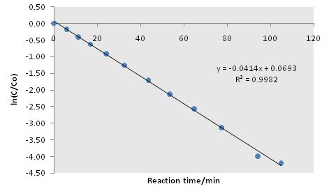
From Figure \(\PageIndex{1}\), we can see that the linearity, i.e., the goodness of the assumption of first order reaction, is very much satisfied throughout the reaction. Thus, the reaction kinetic model is validated. Furthermore, the reaction rate constant can be calculated from the slope of the fitted line, i.e., kmeas = 0.0414 min-1. From this the kcat can be obtained, \ref{4}.
\[ k_{cat}\ =\ k_{meas}/C_{Pd}\ =\ \frac{0.0414min^{-1}{(5 \times 10^{-4}\ g/0.173L)}\ =\ 14.32L/g_{Pd}\ min \label{4} \]