
28.3: Instruments for Liquid Chromatography
- Page ID
- 362585

\( \newcommand{\vecs}[1]{\overset { \scriptstyle \rightharpoonup} {\mathbf{#1}} } \)
\( \newcommand{\vecd}[1]{\overset{-\!-\!\rightharpoonup}{\vphantom{a}\smash {#1}}} \)
\( \newcommand{\id}{\mathrm{id}}\) \( \newcommand{\Span}{\mathrm{span}}\)
( \newcommand{\kernel}{\mathrm{null}\,}\) \( \newcommand{\range}{\mathrm{range}\,}\)
\( \newcommand{\RealPart}{\mathrm{Re}}\) \( \newcommand{\ImaginaryPart}{\mathrm{Im}}\)
\( \newcommand{\Argument}{\mathrm{Arg}}\) \( \newcommand{\norm}[1]{\| #1 \|}\)
\( \newcommand{\inner}[2]{\langle #1, #2 \rangle}\)
\( \newcommand{\Span}{\mathrm{span}}\)
\( \newcommand{\id}{\mathrm{id}}\)
\( \newcommand{\Span}{\mathrm{span}}\)
\( \newcommand{\kernel}{\mathrm{null}\,}\)
\( \newcommand{\range}{\mathrm{range}\,}\)
\( \newcommand{\RealPart}{\mathrm{Re}}\)
\( \newcommand{\ImaginaryPart}{\mathrm{Im}}\)
\( \newcommand{\Argument}{\mathrm{Arg}}\)
\( \newcommand{\norm}[1]{\| #1 \|}\)
\( \newcommand{\inner}[2]{\langle #1, #2 \rangle}\)
\( \newcommand{\Span}{\mathrm{span}}\) \( \newcommand{\AA}{\unicode[.8,0]{x212B}}\)
\( \newcommand{\vectorA}[1]{\vec{#1}} % arrow\)
\( \newcommand{\vectorAt}[1]{\vec{\text{#1}}} % arrow\)
\( \newcommand{\vectorB}[1]{\overset { \scriptstyle \rightharpoonup} {\mathbf{#1}} } \)
\( \newcommand{\vectorC}[1]{\textbf{#1}} \)
\( \newcommand{\vectorD}[1]{\overrightarrow{#1}} \)
\( \newcommand{\vectorDt}[1]{\overrightarrow{\text{#1}}} \)
\( \newcommand{\vectE}[1]{\overset{-\!-\!\rightharpoonup}{\vphantom{a}\smash{\mathbf {#1}}}} \)
\( \newcommand{\vecs}[1]{\overset { \scriptstyle \rightharpoonup} {\mathbf{#1}} } \)
\( \newcommand{\vecd}[1]{\overset{-\!-\!\rightharpoonup}{\vphantom{a}\smash {#1}}} \)
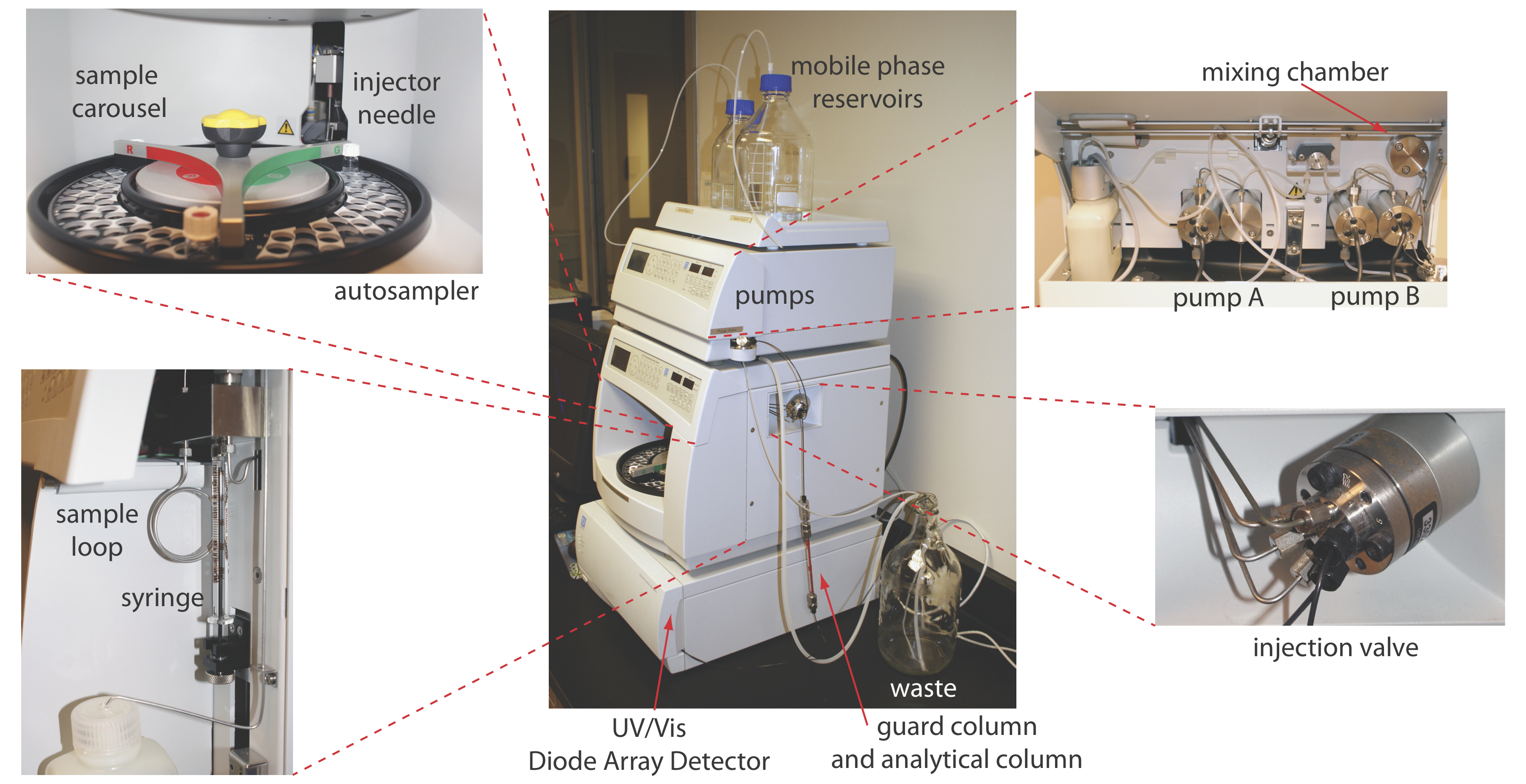
\(\newcommand{\avec}{\mathbf a}\) \(\newcommand{\bvec}{\mathbf b}\) \(\newcommand{\cvec}{\mathbf c}\) \(\newcommand{\dvec}{\mathbf d}\) \(\newcommand{\dtil}{\widetilde{\mathbf d}}\) \(\newcommand{\evec}{\mathbf e}\) \(\newcommand{\fvec}{\mathbf f}\) \(\newcommand{\nvec}{\mathbf n}\) \(\newcommand{\pvec}{\mathbf p}\) \(\newcommand{\qvec}{\mathbf q}\) \(\newcommand{\svec}{\mathbf s}\) \(\newcommand{\tvec}{\mathbf t}\) \(\newcommand{\uvec}{\mathbf u}\) \(\newcommand{\vvec}{\mathbf v}\) \(\newcommand{\wvec}{\mathbf w}\) \(\newcommand{\xvec}{\mathbf x}\) \(\newcommand{\yvec}{\mathbf y}\) \(\newcommand{\zvec}{\mathbf z}\) \(\newcommand{\rvec}{\mathbf r}\) \(\newcommand{\mvec}{\mathbf m}\) \(\newcommand{\zerovec}{\mathbf 0}\) \(\newcommand{\onevec}{\mathbf 1}\) \(\newcommand{\real}{\mathbb R}\) \(\newcommand{\twovec}[2]{\left[\begin{array}{r}#1 \\ #2 \end{array}\right]}\) \(\newcommand{\ctwovec}[2]{\left[\begin{array}{c}#1 \\ #2 \end{array}\right]}\) \(\newcommand{\threevec}[3]{\left[\begin{array}{r}#1 \\ #2 \\ #3 \end{array}\right]}\) \(\newcommand{\cthreevec}[3]{\left[\begin{array}{c}#1 \\ #2 \\ #3 \end{array}\right]}\) \(\newcommand{\fourvec}[4]{\left[\begin{array}{r}#1 \\ #2 \\ #3 \\ #4 \end{array}\right]}\) \(\newcommand{\cfourvec}[4]{\left[\begin{array}{c}#1 \\ #2 \\ #3 \\ #4 \end{array}\right]}\) \(\newcommand{\fivevec}[5]{\left[\begin{array}{r}#1 \\ #2 \\ #3 \\ #4 \\ #5 \\ \end{array}\right]}\) \(\newcommand{\cfivevec}[5]{\left[\begin{array}{c}#1 \\ #2 \\ #3 \\ #4 \\ #5 \\ \end{array}\right]}\) \(\newcommand{\mattwo}[4]{\left[\begin{array}{rr}#1 \amp #2 \\ #3 \amp #4 \\ \end{array}\right]}\) \(\newcommand{\laspan}[1]{\text{Span}\{#1\}}\) \(\newcommand{\bcal}{\cal B}\) \(\newcommand{\ccal}{\cal C}\) \(\newcommand{\scal}{\cal S}\) \(\newcommand{\wcal}{\cal W}\) \(\newcommand{\ecal}{\cal E}\) \(\newcommand{\coords}[2]{\left\{#1\right\}_{#2}}\) \(\newcommand{\gray}[1]{\color{gray}{#1}}\) \(\newcommand{\lgray}[1]{\color{lightgray}{#1}}\) \(\newcommand{\rank}{\operatorname{rank}}\) \(\newcommand{\row}{\text{Row}}\) \(\newcommand{\col}{\text{Col}}\) \(\renewcommand{\row}{\text{Row}}\) \(\newcommand{\nul}{\text{Nul}}\) \(\newcommand{\var}{\text{Var}}\) \(\newcommand{\corr}{\text{corr}}\) \(\newcommand{\len}[1]{\left|#1\right|}\) \(\newcommand{\bbar}{\overline{\bvec}}\) \(\newcommand{\bhat}{\widehat{\bvec}}\) \(\newcommand{\bperp}{\bvec^\perp}\) \(\newcommand{\xhat}{\widehat{\xvec}}\) \(\newcommand{\vhat}{\widehat{\vvec}}\) \(\newcommand{\uhat}{\widehat{\uvec}}\) \(\newcommand{\what}{\widehat{\wvec}}\) \(\newcommand{\Sighat}{\widehat{\Sigma}}\) \(\newcommand{\lt}{<}\) \(\newcommand{\gt}{>}\) \(\newcommand{\amp}{&}\) \(\definecolor{fillinmathshade}{gray}{0.9}\)In high-performance liquid chromatography (HPLC) we inject the sample, which is in solution form, into a liquid mobile phase. The mobile phase carries the sample through a packed or capillary column that separates the sample’s components based on their ability to partition between the mobile phase and the stationary phase. Figure 28.3.1 shows an example of a typical HPLC instrument, which has several key components: reservoirs that store the mobile phase; a pump for pushing the mobile phase through the system; an injector for introducing the sample; a column for separating the sample into its component parts; and a detector for monitoring the eluent as it comes off the column. Let’s consider each of these components.
HPLC Columns
An HPLC typically includes two columns: an analytical column, which is responsible for the separation, and a guard column that is placed before the analytical column to protect it from contamination.
Analytical Columns
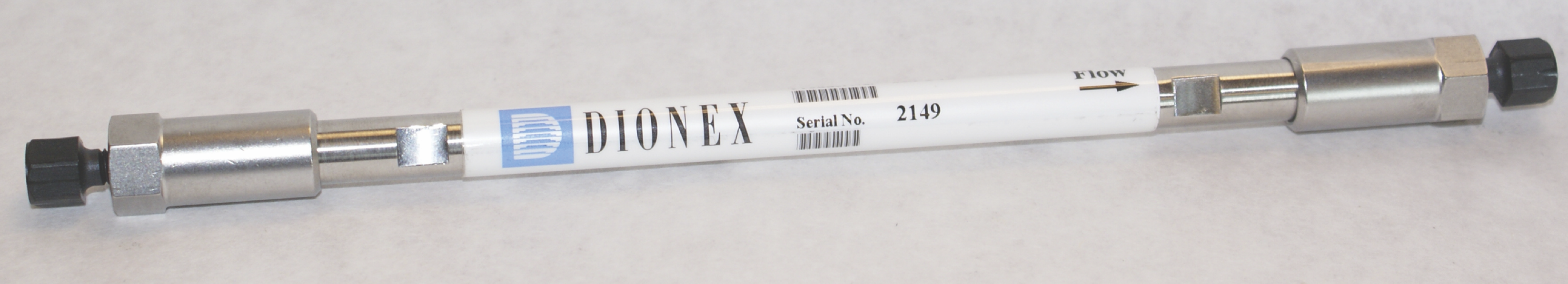
The most common type of HPLC column is a stainless steel tube with an internal diameter between 2.1 mm and 4.6 mm and a length between 30 mm and 300 mm (Figure 28.3.2 ). The column is packed with 3–10 µm porous silica particles with either an irregular or a spherical shape. Typical column efficiencies are 40 000–60 000 theoretical plates/m. A 25-cm column with 50 000 plates/m has 12 500 theoretical plates.
Capillary columns use less solvent and, because the sample is diluted to a lesser extent, produce larger signals at the detector. These columns are made from fused silica capillaries with internal diameters from 44–200 μm and lengths of 50–250 mm. Capillary columns packed with 3–5 μm particles have been prepared with column efficiencies of up to 250 000 theoretical plates [Novotony, M. Science, 1989, 246, 51–57].
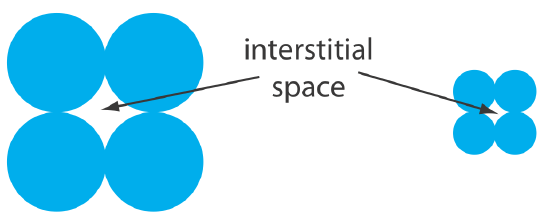
One limitation to a packed capillary column is the back pressure that develops when pumping the mobile phase through the small interstitial spaces between the particulate micron-sized packing material (Figure 28.3.3 ). Because the tubing and the fittings that carry the mobile phase have pressure limits, a higher back pressure requires a lower flow rate and a longer analysis time. Monolithic columns, in which the solid support is a single, porous rod, offer column efficiencies equivalent to a packed capillary column while allowing for faster flow rates. A monolithic column—which usually is similar in size to a conventional packed column, although smaller, capillary columns also are available—is prepared by forming the mono- lithic rod in a mold and covering it with PTFE tubing or a polymer resin. Monolithic rods made of a silica-gel polymer typically have macropores with diameters of approximately 2 μm and mesopores—pores within the macropores—with diameters of approximately 13 nm [Cabrera, K. Chromatography Online, April 1, 2008].
Guard Columns
Two problems tend to shorten the lifetime of an analytical column. First, solutes that bind irreversibly to the stationary phase degrade the column’s performance by decreasing the amount of stationary phase available for effecting a separation. Second, particulate material injected with the sample may clog the analytical column. To minimize these problems we place a guard column before the analytical column. A guard column usually contains the same particulate packing material and stationary phase as the analytical column, but is significantly shorter and less expensive—a length of 7.5 mm and a cost one-tenth of that for the corresponding analytical column is typical. Because they are intended to be sacrificial, guard columns are replaced regularly. If you look closely at Figure 28.3.1 , you will see the small guard column just above the analytical column.
HPLC Plumbing
In a gas chromatograph the pressure from a compressed gas cylinder is sufficient to push the mobile phase through the column. Pushing a liquid mobile phase through a column, however, takes a great deal more effort, generating pressures in excess of several hundred atmospheres. In this section we consider the basic plumbing needed to move the mobile phase through the column and to inject the sample into the mobile phase.
Moving the Mobile Phase
A typical HPLC includes between 1–4 reservoirs for storing mobile phase solvents. The instrument in Figure 28.3.1 , for example, has two mobile phase reservoirs that are used for an isocratic elution or a gradient elution by drawing solvents from one or both reservoirs.
Before using a mobile phase solvent we must remove dissolved gases, such as N2 and O2, and small particulate matter, such as dust. Because there is a large drop in pressure across the column—the pressure at the column’s entrance is as much as several hundred atmospheres, but it is atmospheric pressure at the column’s exit—gases dissolved in the mobile phase are released as gas bubbles that may interfere with the detector’s response. Degassing is accomplished in several ways, but the most common are the use of a vacuum pump or sparging with an inert gas, such as He, which has a low solubility in the mobile phase. Particulate materials, which may clog the HPLC tubing or column, are removed by filtering the solvents.
Bubbling an inert gas through the mobile phase releases volatile dissolved gases. This process is called sparging.
The mobile phase solvents are pulled from their reservoirs by the action of one or more pumps. Figure 28.3.4 shows a close-up view of the pumps for the instrument in Figure 28.3.1 . The working pump and the equilibrating pump each have a piston whose back and forth movement maintains a constant flow rate of up to several mL/min and provides the high output pressure needed to push the mobile phase through the chromatographic column. In this particular instrument, each pump sends its mobile phase to a mixing chamber where they combine to form the final mobile phase. The relative speed of the two pumps determines the mobile phase’s final composition.
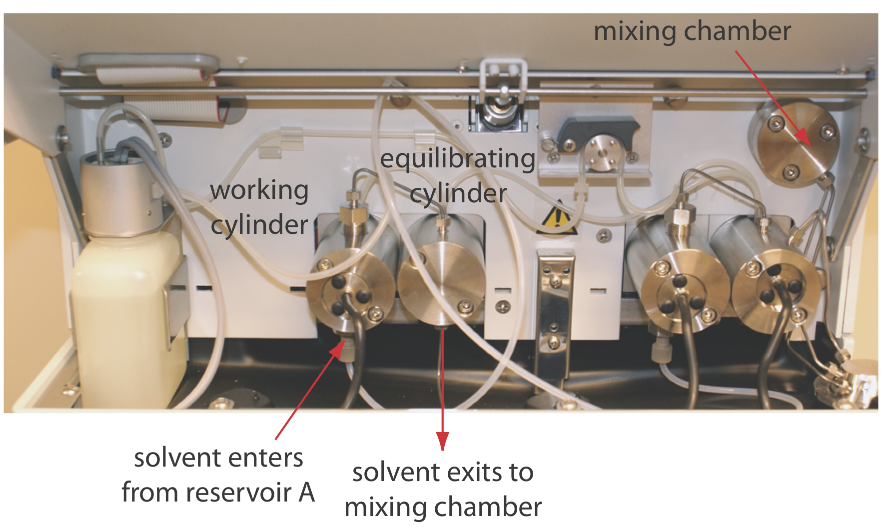
The back and forth movement of a reciprocating pump creates a pulsed flow that contributes noise to the chromatogram. To minimize these pulses, each pump in Figure 28.3.4 has two cylinders. During the working cylinder’s forward stoke it fills the equilibrating cylinder and establishes flow through the column. When the working cylinder is on its reverse stroke, the flow is maintained by the piston in the equilibrating cylinder. The result is a pulse-free flow.
There are other ways to control the mobile phase’s composition and flow rate. For example, instead of the two pumps in Figure 28.3.4 , we can place a solvent proportioning valve before a single pump. The solvent proportioning value connects two or more solvent reservoirs to the pump and determines how much of each solvent is pulled during each of the pump’s cycles. Another approach for eliminating a pulsed flow is to include a pulse damper between the pump and the column. A pulse damper is a chamber filled with an easily compressed fluid and a flexible diaphragm. During the piston’s forward stroke the fluid in the pulse damper is compressed. When the piston withdraws to refill the pump, pressure from the expanding fluid in the pulse damper maintains the flow rate.
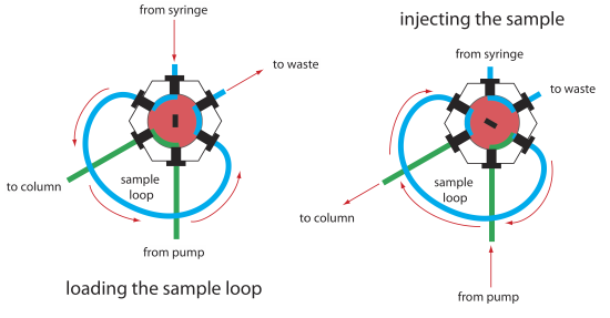
Injecting the Sample
The operating pressure within an HPLC is sufficiently high that we cannot inject the sample into the mobile phase by inserting a syringe through a septum, as is possible in gas chromatography. Instead, we inject the sample using a loop injector, a diagram of which is shown in Figure 28.3.5 . In the load position a sample loop—which is available in a variety of sizes ranging from 0.5 μL to 5 mL—is isolated from the mobile phase and open to the atmosphere. The sample loop is filled using a syringe with a capacity several times that of the sample loop, with excess sample exiting through the waste line. After loading the sample, the injector is turned to the inject position, which redirects the mobile phase through the sample loop and onto the column.
The instrument in Figure 28.3.1 uses an autosampler to inject samples. Instead of using a syringe to push the sample into the sample loop, the syringe draws sample into the sample loop.
Detectors for HPLC
Many different types of detectors have been use to monitor HPLC separations, most of which use spectroscopy or electrochemistry to generate a measurable signal.
Spectroscopic Detectors
The most popular HPLC detectors take advantage of an analyte’s UV/Vis absorption spectrum. These detectors range from simple designs, in which the analytical wavelength is selected using appropriate filters, to a modified spectrophotometer in which the sample compartment includes a flow cell. Figure 28.3.6 shows the design of a typical flow cell when using a diode array spectrometer as the detector. The flow cell has a volume of 1–10 μL and a path length of 0.2–1 cm.
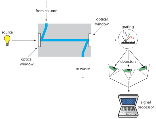
When using a UV/Vis detector the resulting chromatogram is a plot of absorbance as a function of elution time. If the detector is a diode array spectrometer, then we also can display the result as a three-dimensional chromatogram that shows absorbance as a function of wavelength and elution time. One limitation to using absorbance is that the mobile phase cannot absorb at the wavelengths we wish to monitor. Absorbance detectors provide detection limits of as little as 100 pg–1 ng of injected analyte. If an analyte is fluorescent, we can place the flow cell in a spectrofluorimeter. Detection limits are as little as 1–10 pg of injected analyte.
Electrochemical Detectors
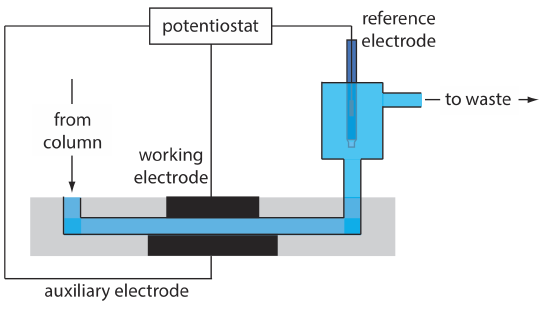
Another common group of HPLC detectors are those based on electrochemical measurements such as amperometry, voltammetry, coulometry, and conductivity. Figure 28.3.7 , for example, shows an amperometric flow cell. Effluent from the column passes over the working electrode—held at a constant potential relative to a downstream reference electrode—that completely oxidizes or reduces the analytes. The current flowing between the working electrode and the auxiliary electrode serves as the analytical signal. Detection limits for amperometric electrochemical detection are from 10 pg–1 ng of injected analyte.
Other Detectors
Several other detectors have been used in HPLC. Measuring a change in the mobile phase’s refractive index is analogous to monitoring the mobile phase’s thermal conductivity in gas chromatography. A refractive index detector is nearly universal, responding to almost all compounds, but has a relatively poor detection limit of 0.1–1 μg of injected analyte. An additional limitation of a refractive index detector is that it cannot be used for a gradient elution unless the mobile phase components have identical refractive indexes.
Another useful detector is a mass spectrometer. Figure 28.3.8 shows a block diagram of a typical HPLC–MS instrument. The effluent from the column enters the mass spectrometer’s ion source using an interface the removes most of the mobile phase, an essential need because of the incompatibility between the liquid mobile phase and the mass spectrometer’s high vacuum environment. In the ionization chamber the remaining molecules—a mixture of the mobile phase components and solutes—undergo ionization and fragmentation. The mass spectrometer’s mass analyzer separates the ions by their mass-to-charge ratio (m/z). A detector counts the ions and displays the mass spectrum.
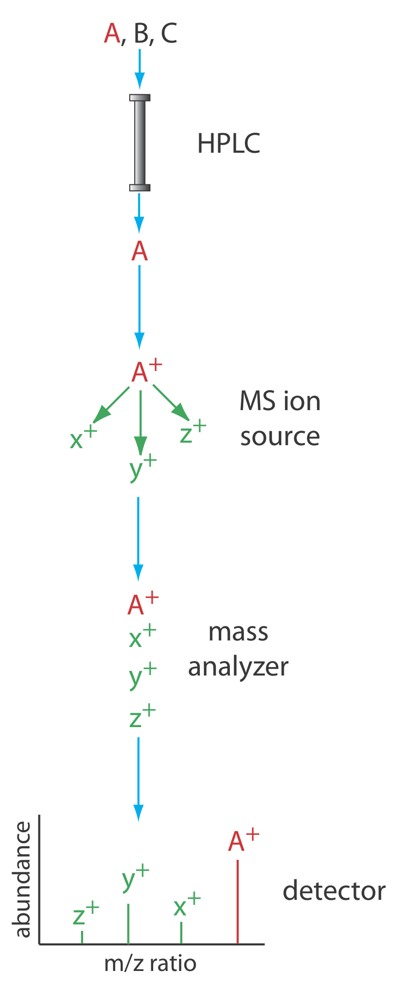
There are several options for monitoring the chromatogram when using a mass spectrometer as the detector. The most common method is to continuously scan the entire mass spectrum and report the total signal for all ions reaching the detector during each scan. This total ion scan provides universal detection for all analytes. We can achieve some degree of selectivity by monitoring only specific mass-to-charge ratios, a process called selective-ion monitoring. The advantages of using a mass spectrometer in HPLC are the same as for gas chromatography. Detection limits are very good, typically 0.1–1 ng of injected analyte, with values as low as 1–10 pg for some samples. In addition, a mass spectrometer provides qualitative, structural information that can help to identify the analytes. The interface between the HPLC and the mass spectrometer is technically more difficult than that in a GC–MS because of the incompatibility of a liquid mobile phase with the mass spectrometer’s high vacuum requirement.