25.2: Voltammetric Instrumentation
- Page ID
- 335295

\( \newcommand{\vecs}[1]{\overset { \scriptstyle \rightharpoonup} {\mathbf{#1}} } \)
\( \newcommand{\vecd}[1]{\overset{-\!-\!\rightharpoonup}{\vphantom{a}\smash {#1}}} \)
\( \newcommand{\dsum}{\displaystyle\sum\limits} \)
\( \newcommand{\dint}{\displaystyle\int\limits} \)
\( \newcommand{\dlim}{\displaystyle\lim\limits} \)
\( \newcommand{\id}{\mathrm{id}}\) \( \newcommand{\Span}{\mathrm{span}}\)
( \newcommand{\kernel}{\mathrm{null}\,}\) \( \newcommand{\range}{\mathrm{range}\,}\)
\( \newcommand{\RealPart}{\mathrm{Re}}\) \( \newcommand{\ImaginaryPart}{\mathrm{Im}}\)
\( \newcommand{\Argument}{\mathrm{Arg}}\) \( \newcommand{\norm}[1]{\| #1 \|}\)
\( \newcommand{\inner}[2]{\langle #1, #2 \rangle}\)
\( \newcommand{\Span}{\mathrm{span}}\)
\( \newcommand{\id}{\mathrm{id}}\)
\( \newcommand{\Span}{\mathrm{span}}\)
\( \newcommand{\kernel}{\mathrm{null}\,}\)
\( \newcommand{\range}{\mathrm{range}\,}\)
\( \newcommand{\RealPart}{\mathrm{Re}}\)
\( \newcommand{\ImaginaryPart}{\mathrm{Im}}\)
\( \newcommand{\Argument}{\mathrm{Arg}}\)
\( \newcommand{\norm}[1]{\| #1 \|}\)
\( \newcommand{\inner}[2]{\langle #1, #2 \rangle}\)
\( \newcommand{\Span}{\mathrm{span}}\) \( \newcommand{\AA}{\unicode[.8,0]{x212B}}\)
\( \newcommand{\vectorA}[1]{\vec{#1}} % arrow\)
\( \newcommand{\vectorAt}[1]{\vec{\text{#1}}} % arrow\)
\( \newcommand{\vectorB}[1]{\overset { \scriptstyle \rightharpoonup} {\mathbf{#1}} } \)
\( \newcommand{\vectorC}[1]{\textbf{#1}} \)
\( \newcommand{\vectorD}[1]{\overrightarrow{#1}} \)
\( \newcommand{\vectorDt}[1]{\overrightarrow{\text{#1}}} \)
\( \newcommand{\vectE}[1]{\overset{-\!-\!\rightharpoonup}{\vphantom{a}\smash{\mathbf {#1}}}} \)
\( \newcommand{\vecs}[1]{\overset { \scriptstyle \rightharpoonup} {\mathbf{#1}} } \)
\(\newcommand{\longvect}{\overrightarrow}\)
\( \newcommand{\vecd}[1]{\overset{-\!-\!\rightharpoonup}{\vphantom{a}\smash {#1}}} \)
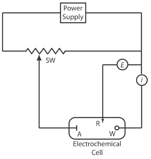
\(\newcommand{\avec}{\mathbf a}\) \(\newcommand{\bvec}{\mathbf b}\) \(\newcommand{\cvec}{\mathbf c}\) \(\newcommand{\dvec}{\mathbf d}\) \(\newcommand{\dtil}{\widetilde{\mathbf d}}\) \(\newcommand{\evec}{\mathbf e}\) \(\newcommand{\fvec}{\mathbf f}\) \(\newcommand{\nvec}{\mathbf n}\) \(\newcommand{\pvec}{\mathbf p}\) \(\newcommand{\qvec}{\mathbf q}\) \(\newcommand{\svec}{\mathbf s}\) \(\newcommand{\tvec}{\mathbf t}\) \(\newcommand{\uvec}{\mathbf u}\) \(\newcommand{\vvec}{\mathbf v}\) \(\newcommand{\wvec}{\mathbf w}\) \(\newcommand{\xvec}{\mathbf x}\) \(\newcommand{\yvec}{\mathbf y}\) \(\newcommand{\zvec}{\mathbf z}\) \(\newcommand{\rvec}{\mathbf r}\) \(\newcommand{\mvec}{\mathbf m}\) \(\newcommand{\zerovec}{\mathbf 0}\) \(\newcommand{\onevec}{\mathbf 1}\) \(\newcommand{\real}{\mathbb R}\) \(\newcommand{\twovec}[2]{\left[\begin{array}{r}#1 \\ #2 \end{array}\right]}\) \(\newcommand{\ctwovec}[2]{\left[\begin{array}{c}#1 \\ #2 \end{array}\right]}\) \(\newcommand{\threevec}[3]{\left[\begin{array}{r}#1 \\ #2 \\ #3 \end{array}\right]}\) \(\newcommand{\cthreevec}[3]{\left[\begin{array}{c}#1 \\ #2 \\ #3 \end{array}\right]}\) \(\newcommand{\fourvec}[4]{\left[\begin{array}{r}#1 \\ #2 \\ #3 \\ #4 \end{array}\right]}\) \(\newcommand{\cfourvec}[4]{\left[\begin{array}{c}#1 \\ #2 \\ #3 \\ #4 \end{array}\right]}\) \(\newcommand{\fivevec}[5]{\left[\begin{array}{r}#1 \\ #2 \\ #3 \\ #4 \\ #5 \\ \end{array}\right]}\) \(\newcommand{\cfivevec}[5]{\left[\begin{array}{c}#1 \\ #2 \\ #3 \\ #4 \\ #5 \\ \end{array}\right]}\) \(\newcommand{\mattwo}[4]{\left[\begin{array}{rr}#1 \amp #2 \\ #3 \amp #4 \\ \end{array}\right]}\) \(\newcommand{\laspan}[1]{\text{Span}\{#1\}}\) \(\newcommand{\bcal}{\cal B}\) \(\newcommand{\ccal}{\cal C}\) \(\newcommand{\scal}{\cal S}\) \(\newcommand{\wcal}{\cal W}\) \(\newcommand{\ecal}{\cal E}\) \(\newcommand{\coords}[2]{\left\{#1\right\}_{#2}}\) \(\newcommand{\gray}[1]{\color{gray}{#1}}\) \(\newcommand{\lgray}[1]{\color{lightgray}{#1}}\) \(\newcommand{\rank}{\operatorname{rank}}\) \(\newcommand{\row}{\text{Row}}\) \(\newcommand{\col}{\text{Col}}\) \(\renewcommand{\row}{\text{Row}}\) \(\newcommand{\nul}{\text{Nul}}\) \(\newcommand{\var}{\text{Var}}\) \(\newcommand{\corr}{\text{corr}}\) \(\newcommand{\len}[1]{\left|#1\right|}\) \(\newcommand{\bbar}{\overline{\bvec}}\) \(\newcommand{\bhat}{\widehat{\bvec}}\) \(\newcommand{\bperp}{\bvec^\perp}\) \(\newcommand{\xhat}{\widehat{\xvec}}\) \(\newcommand{\vhat}{\widehat{\vvec}}\) \(\newcommand{\uhat}{\widehat{\uvec}}\) \(\newcommand{\what}{\widehat{\wvec}}\) \(\newcommand{\Sighat}{\widehat{\Sigma}}\) \(\newcommand{\lt}{<}\) \(\newcommand{\gt}{>}\) \(\newcommand{\amp}{&}\) \(\definecolor{fillinmathshade}{gray}{0.9}\)Although early voltammetric methods used only two electrodes, a modern voltammeter makes use of a three-electrode potentiostat, such as that shown in Figure \(\PageIndex{1}\). The potential of the working electrode is measured relative to a constant-potential reference electrode that is connected to the working electrode through a high-impedance potentiometer. The auxiliary electrode generally is a platinum wire and the reference electrode usually is a SCE or a Ag/AgCl electrode. We apply a time-dependent potential excitation signal to the working electrode—changing its potential relative to the fixed potential of the reference electrode—and measure the current that flows between the working electrode and the auxiliary electrode. Modern potentiostats include waveform generators that allow us to apply a time-dependent potential profile, such as a series of potential pulses, to the working electrode.
Working Electrodes
For the working electrode we can choose among several different materials, including mercury, platinum, gold, silver, and carbon. The earliest voltammetric techniques used a mercury working electrode. Because mercury is a liquid, the working electrode usually is a drop suspended from the end of a capillary tube. In the hanging mercury drop electrode, or HMDE, we extrude the drop of Hg by rotating a micrometer screw that pushes the mercury from a reservoir through a narrow capillary tube (Figure \(\PageIndex{2}\)a).
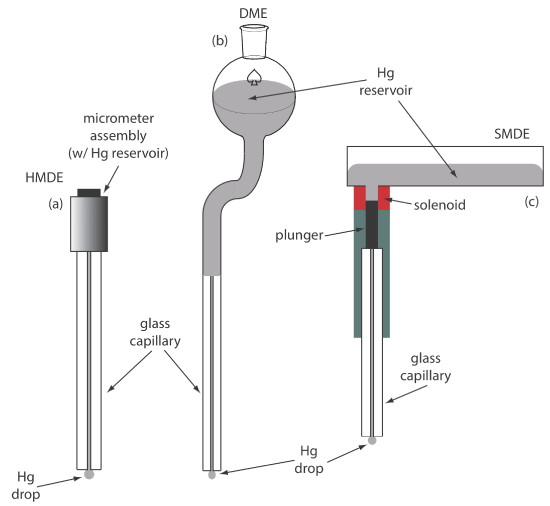
In the dropping mercury electrode, or DME, mercury drops form at the end of the capillary tube as a result of gravity (Figure \(\PageIndex{2}\)b). Unlike the HMDE, the mercury drop of a DME grows continuously—as mercury flows from the reservoir under the influence of gravity—and has a finite lifetime of several seconds. At the end of its lifetime the mercury drop is dislodged, either manually or on its own, and is replaced by a new drop. The static mercury drop electrode, or SMDE, uses a solenoid driven plunger to control the flow of mercury (Figure \(\PageIndex{2}\)c). Activation of the solenoid momentarily lifts the plunger, allowing mercury to flow through the capillary, forming a single, hanging Hg drop. Repeated activation of the solenoid produces a series of Hg drops. In this way the SMDE may be used as either a HMDE or a DME. There is one additional type of mercury electrode: the mercury film electrode. A solid electrode—typically carbon, platinum, or gold—is placed in a solution of Hg2+ and held at a potential where the reduction of Hg2+ to Hg is favorable, depositing a thin film of mercury on the solid electrode’s surface.
Mercury has several advantages as a working electrode. Perhaps its most important advantage is its high overpotential for the reduction of H3O+ to H2, which makes accessible potentials as negative as –1 V versus the SCE in acidic solutions and –2 V versus the SCE in basic solutions (Figure \(\PageIndex{3}\)). A species such as Zn2+, which is difficult to reduce at other electrodes without simultaneously reducing H3O+, is easy to reduce at a mercury working electrode. Other advantages include the ability of metals to dissolve in mercury—which results in the formation of an amalgam—and the ability to renew the surface of the electrode by extruding a new drop. One limitation to mercury as a working electrode is the ease with which it is oxidized. Depending on the solvent, a mercury electrode can not be used at potentials more positive than approximately –0.3 V to +0.4 V versus the SCE.
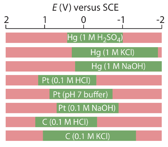
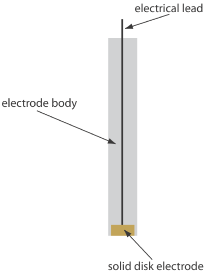
Solid electrodes constructed using platinum, gold, silver, or carbon may be used over a range of potentials, including potentials that are negative and positive with respect to the SCE (Figure \(\PageIndex{3}\)). For example, the potential window for a Pt electrode extends from approximately +1.2 V to –0.2 V versus the SCE in acidic solutions, and from +0.7 V to –1 V versus the SCE in basic solutions. A solid electrode can replace a mercury electrode for many voltammetric analyses that require negative potentials, and is the electrode of choice at more positive potentials. Except for the carbon paste electrode, a solid electrode is fashioned into a disk and sealed into the end of an inert support with an electrical lead (Figure \(\PageIndex{4}\)). The carbon paste electrode is made by filling the cavity at the end of the inert support with a paste that consists of carbon particles and a viscous oil. Solid electrodes are not without problems, the most important of which is the ease with which the electrode’s surface is altered by the adsorption of a solution species or by the formation of an oxide layer. For this reason a solid electrode needs frequent reconditioning, either by applying an appropriate potential or by polishing.
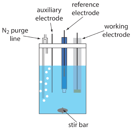
Electrochemical Cells
A typical arrangement for a voltammetric electrochemical cell is shown in Figure \(\PageIndex{5}\). In addition to the working electrode, the reference electrode, and the auxiliary electrode, the cell also includes a N2-purge line for removing dissolved O2, and an optional stir bar. Electrochemical cells are available in a variety of sizes, allowing the analysis of solution volumes ranging from more than 100 mL to as small as 50 μL.