25.3: Linear Sweep Voltammetry

In the simplest voltammetric experiment we apply a linear potential ramp as an excitation signal and record the current that flows in response to the change in potential. Among the experimental variables under our control are the initial potential, the final potential, the scan rate, and whether we choose to stir the solution or leave it unstirred. We call this linear sweep voltammetry.

To illustrate how linear sweep voltammetry works, let's consider what happens when we reduce \(\text{Fe(CN)}_6^{3-}\) to \(\text{Fe(CN)}_6^{4-}\) at the working electrode. The relationship between the concentrations of \(\text{Fe(CN)}_6^{3-}\), the concentration of \(\text{Fe(CN)}_6^{4-}\), and the potential is given by the Nernst equation

\[E=+0.356 \text{ V}-0.05916 \log \frac{\left[\mathrm{Fe}(\mathrm{CN})_{6}^{4-}\right]_{x=0}}{\left[\mathrm{Fe}(\mathrm{CN})_{6}^{3-}\right]_{x=0}} \label{lsv1} \]

where +0.356V is the standard-state potential for the \(\text{Fe(CN)}_6^{3-}\)/\(\text{Fe(CN)}_6^{4-}\) redox couple, and x = 0 indicates that the concentrations of \(\text{Fe(CN)}_6^{3-}\) and \(\text{Fe(CN)}_6^{4-}\) are those at the surface of the working electrode. We use surface concentrations instead of bulk concentrations because the equilibrium position for the redox reaction

\[\mathrm{Fe}(\mathrm{CN})_{6}^{3-}(a q)+e^{-}\rightleftharpoons\mathrm{Fe}(\mathrm{CN})_{6}^{4-}(a q) \label{lsv2} \]

is established at the electrode’s surface.

Let’s assume we have a solution for which the initial concentration of \(\text{Fe(CN)}_6^{3-}\) is 1.0 mM and that \(\text{Fe(CN)}_6^{4-}\) is absent. Figure \(\PageIndex{1}\) shows the relationship between the applied potential and the species that are stable at the electrode's surface.

Figure \(\PageIndex{1}\). Potential diagram for the \(\text{Fe(CN)}_6^{3-}\)/\(\text{Fe(CN)}_6^{4-}\) redox half-reaction showing the potentials where \(\text{Fe(CN)}_6^{3-}\) and where \(\text{Fe(CN)}_6^{4-}\) are the dominate species. At a potential of +0.30 V, only \(\text{Fe(CN)}_6^{3-}\) is stable at the electrode's surface.

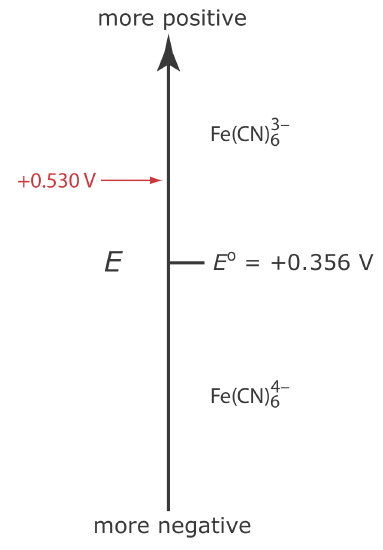
If we apply a potential of +0.530 V to the working electrode, the concentrations of \(\text{Fe(CN)}_6^{3-}\) and \(\text{Fe(CN)}_6^{4-}\) at the surface of the electrode are unaffected, and no faradaic current is observed. If we switch the potential to +0.356 V some of the \(\text{Fe(CN)}_6^{3-}\) at the electrode’s surface is reduced to \(\text{Fe(CN)}_6^{4-}\)until we reach a condition where

\[\left[\mathrm{Fe}(\mathrm{CN})_{6}^{3-}\right]_{x=0}=\left[\mathrm{Fe}(\mathrm{CN})_{6}^{4-}\right]_{x=0}=0.50 \text{ mM} \label{lsv3} \]

If this is all that happens after we apply the potential, then there would be a brief surge of faradaic current that quickly returns to zero, which is not the most interesting of results (although this is the basis for chronoamperometry, an electrochemical method we will not consider in this text). Although the concentrations of \(\text{Fe(CN)}_6^{3-}\) and \(\text{Fe(CN)}_6^{4-}\) at the electrode surface are 0.50 mM, their concentrations in bulk solution remains unchanged.

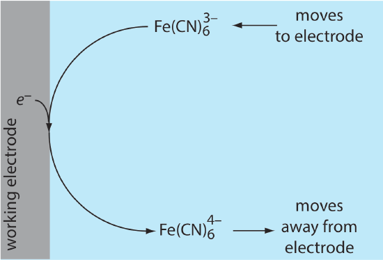
Because of this difference in concentration, there is a concentration gradient between the electrode’s surface and the bulk solution. This concentration gradient creates a driving force that transports \(\text{Fe(CN)}_6^{4-}\) away from the electrode and that transports \(\text{Fe(CN)}_6^{3-}\) to the electrode (Figure \(\PageIndex{2}\)). As the \(\text{Fe(CN)}_6^{3-}\) arrives at the electrode it, too, is reduced to \(\text{Fe(CN)}_6^{4-}\). A faradaic current continues to flow until there is no difference between the concentrations of \(\text{Fe(CN)}_6^{3-}\) and \(\text{Fe(CN)}_6^{4-}\) at the electrode and their concentrations in bulk solution (although this might take a long time!).

Figure \(\PageIndex{2}\). Schematic diagram showing the transport of \(\text{Fe(CN)}_6^{4-}\) away from the electrode’s surface and the transport of \(\text{Fe(CN)}_6^{3-}\) toward the electrode’s surface following the reduction of \(\text{Fe(CN)}_6^{3-}\) to \(\text{Fe(CN)}_6^{4-}\).

Although the potential at the working electrode determines if a faradaic current flows, the magnitude of the current is determined by the rate of the resulting oxidation or reduction reaction. Two factors contribute to the rate of the electrochemical reaction: the rate at which the reactants and products are transported to and from the electrode—what we call mass transport—and the rate at which electrons pass between the electrode and the reactants and products in solution.

Concentration Profiles at the Working Electrode

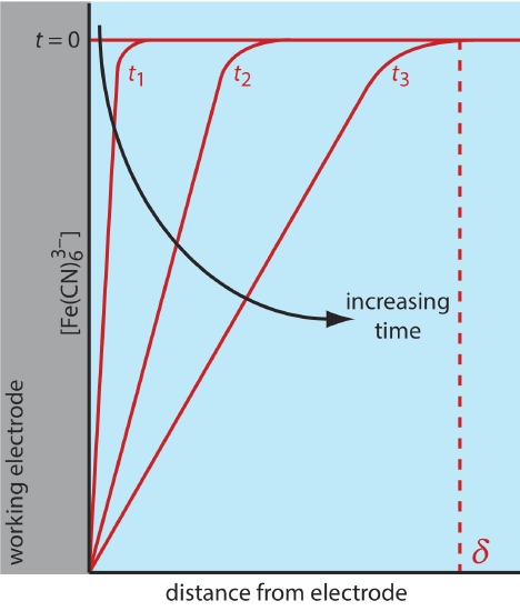
There are three modes of mass transport that affect the rate at which reactants and products move toward or away from the electrode surface: diffusion, migration, and convection. Diffusion occurs whenever the concentration of an ion or a molecule at the surface of the electrode is different from that in bulk solution. If we apply a potential sufficient to completely reduce \(\text{Fe(CN)}_6^{3-}\) at the electrode surface, the result is a concentration gradient similar to that shown in Figure \(\PageIndex{3}\). The region of solution over which diffusion occurs is the diffusion layer. In the absence of other modes of mass transport, the width of the diffusion layer, \(\delta\), increases with time as the \(\text{Fe(CN)}_6^{3-}\) must diffuse from an increasingly greater distance.

Figure \(\PageIndex{3}\). Concentration gradients (in red) for \(\text{Fe(CN)}_6^{3-}\) following the application of a potential that completely reduces it to \(\text{Fe(CN)}_6^{4-}\). Before we apply the potential (t = 0) the concentration of \(\text{Fe(CN)}_6^{3-}\) is the same at all distances from the electrode’s surface. After we apply the potential, its concentration at the electrode’s surface decreases to zero and \(\text{Fe(CN)}_6^{3-}\) diffuses to the electrode from bulk solution. The longer we apply the potential, the greater the distance over which diffusion occurs. The dashed red line shows the extent of the diffusion layer at time t₃. These profiles assume that convection and migration do not contribute significantly to the mass transport of \(\text{Fe(CN)}_6^{3-}\).

Convection occurs when we mix the solution, which carries reactants toward the electrode and removes products from the electrode. The most common form of convection is stirring the solution with a stir bar; other methods include rotating the electrode and incorporating the electrode into a flow-cell.

The final mode of mass transport is migration, which occurs when a charged particle in solution is attracted to or repelled from an electrode that carries a surface charge. If the electrode carries a positive charge, for example, an anion will move toward the electrode and a cation will move toward the bulk solution. Unlike diffusion and convection, migration affects only the mass transport of charged particles.

The movement of material to and from the electrode surface is a complex function of all three modes of mass transport. In the limit where diffusion is the only significant form of mass transport, the current, \(i\), in a voltammetric cell is proportional to the slope of the concentration profile in Figure \(\PageIndex{3}\)

\[i \propto \frac {\partial C} {\partial x} \label{lsv4} \]

where \(C\) is the concentration of \(\text{Fe(CN)}_6^{3-}\) and \(x\) is distance.

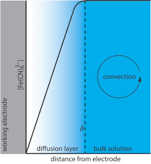
For Equation \ref{lsv4} to be valid, convection and migration must not interfere with the formation of a diffusion layer. We can eliminate migration by adding a high concentration of an inert supporting electrolyte. Because ions of similar charge are equally attracted to or repelled from the surface of the electrode, each has an equal probability of undergoing migration. A large excess of an inert electrolyte ensures that few reactants or products experience migration. Although it is easy to eliminate convection by not stirring the solution, there are experimental designs where we cannot avoid convection, either because we must stir the solution or because we are using an electrochemical flow cell. Fortunately, as shown in Figure \(\PageIndex{4}\), the dynamics of a fluid moving past an electrode results in a small diffusion layer—typically 1–10 μm in thickness—in which the rate of mass transport by convection drops to zero.

Figure \(\PageIndex{4}\). Concentration gradient for \(\text{Fe(CN)}_6^{3-}\) when stirring the solution. Diffusion is the only significant form of mass transport close to the electrode’s surface. At distances greater than \(\delta\), convection is the only significant form of mass transport, maintaining a homogeneous solution in which the concentration of \(\text{Fe(CN)}_6^{3-}\) at \(\delta\) is the same as its concentration in bulk solution.

Concentration Profiles in an Unstirred Solution

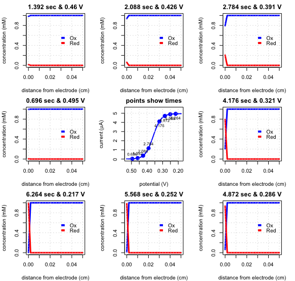
Figure \(\PageIndex{5}\) shows the linear sweep voltammogram (the center image, which shows the current as a function of time) and eight snapshots of the concentration profiles for the reduction of \(\text{Fe(CN)}_6^{3-}\) to \(\text{Fe(CN)}_6^{4-}\) in an unstirred solution. The initial potential was set to +0.530 V and the final potential was set to +0.182 V with a scan rate of 0.050 V/s.

At the initial potential, only \(\text{Fe(CN)}_6^{3-}\) is stable at the electrode surface, and no current flows. After 0.696 s the potential is 0.495 V (image to the left of the linear sweep voltammogram) and, because \(\text{Fe(CN)}_6^{3-}\) remains stable at the electrode surface, no current flows. Moving clockwise around the linear sweep voltammogram, the applied potential becomes smaller and the concentration of \(\text{Fe(CN)}_6^{3-}\) at the electrode surface decreases and the concentration of \(\text{Fe(CN)}_6^{4-}\) increases. Initially the slope of the concentration gradient, and, therefore, the current increases; as the concentration of \(\text{Fe(CN)}_6^{3-}\) at the electrode surface approaches zero, however, the concentration gradient becomes less steep and the current decreases. The result is the linear sweep voltammogram in the center of the diagram.

Figure \(\PageIndex{5}\): The central image shows the linear sweep voltammogram in an unstirred solution for the reduction of \(\text{Fe(CN)}_6^{3-}\) to \(\text{Fe(CN)}_6^{4-}\). The remaining images show the concentration profiles for \(\text{Fe(CN)}_6^{3-}\) (in blue) and for \(\text{Fe(CN)}_6^{4-}\) (in red) as the potential is swept from +0.530 V to +0.182 V (arranged clockwise, beginning immediately left of the linear sweep voltammogram.

Concentration Profiles in a Stirred Solution

If we run the same experiment as in Figure \(\PageIndex{5}\), but stir the solution, the resulting linear sweep voltammogram and concentration profiles are those in Figure \(\PageIndex{6}\). Stirring the solution, as we saw in Figure \(\PageIndex{4}\) creates a diffusion layer whose thickness is independent of time.

Figure \(\PageIndex{6}\): The central image shows the linear sweep voltammogram in a stirred solution for the reduction of \(\text{Fe(CN)}_6^{3-}\) to \(\text{Fe(CN)}_6^{4-}\). The remaining images show the concentration profiles for \(\text{Fe(CN)}_6^{3-}\) (in blue) and for \(\text{Fe(CN)}_6^{4-}\) (in red) as the potential is swept from +0.530 V to +0.182 V (arranged clockwise, beginning immediately left of the linear sweep voltammogram.

As a result, instead of the peak current in Figure \(\PageIndex{5}\), the current reaches a steady-state value, which we call the limiting current, \(i_l\). The linear sweep voltammogram also has a characteristic half-wave potential, \(E_{1/2}\), when the current is 50% of the limiting current. Figure \(\PageIndex{7}\) shows how the limiting current and half-wave potential are measured.

Figure \(\PageIndex{7}\): The limiting current and half-wave potential for a linear sweep voltammetry experiment in a stirred solution.

Voltammetric Currents

Earlier we noted, in Equation \ref{lsv4}, that the current in linear sweep voltammetry is proportional to the slope of the concentration profile. The current is also a function of other variables, as shown here for the reduction of \(\text{Fe(CN)}_6^{3-}\) to \(\text{Fe(CN)}_6^{4-}\)

\[i = \frac{ n F A D \left( \left[ \ce{Fe(CN)6^{3-}} \right]_\text{bulk} - \left[ \ce{Fe(CN)6^{3-}} \right]_\text{x = 0} \right)} {\delta} \label{lsv5} \]

where n the number of electrons in the redox reaction, F is Faraday’s constant, A is the area of the electrode, D is the diffusion coefficient for \(\text{Fe(CN)}_6^{3-}\), \(\delta\) is the thickness of the diffusion layer, and \(\left( \left[ \ce{Fe(CN)6^{3-}} \right]_\text{bulk} - \left[ \ce{Fe(CN)6^{3-}} \right]_\text{x = 0} \right)\) is the difference in the concentration of \( \ce{Fe(CN)6^{3-}}\) between the bulk solution and the electrode's surface.

Because \(n\), \(F\), \(A\), and \(D\) are constants, and because \(\delta\) is a constant if we stir the solution, we can write Equation \ref{lsv5} as

\[i = K_{\ce{Fe(CN)6^{3-}}} \left( \left[ \ce{Fe(CN)6^{3-}} \right]_\text{bulk} - \left[ \ce{Fe(CN)6^{3-}} \right]_\text{x = 0} \right) \label{lsv6} \]

where \(K_{\ce{Fe(CN)6^{3-}}}\) is a constant. If we use the limiting current, then \(\left[ \ce{Fe(CN)6^{3-}} \right]_\text{x = 0}\) is zero, and Equation \ref{lsv6} becomes

\[i_l = K_{\ce{Fe(CN)6^{3-}}} \left[ \ce{Fe(CN)6^{3-}} \right]_\text{bulk} \label{lsv7} \]

Current/Voltage Relationships for Reversible Reactions

A reversible electrochemical reaction is one in which the concentration of the oxidized and reduced species at the electrode surface remain in thermodynamic equilibrium with each other. When this is true, the Nernst equation explains the relationship between the applied potential, their concentration, and the standard state potential.

Equation \ref{lsv7} shows us that the limiting current is a measure of the concentration of \(\text{Fe(CN)}_6^{3-}\) in bulk solution, which means we can use the limiting current for quantitative work. Figure \(\PageIndex{7}\) also shows that there is a qualitative relationship between the half-wave potential, \(E_{1/2}\), and the limiting current; however, it is not yet clear what the half-wave potential represents.

If we solve Equation \ref{lsv7} for \(\left[ \ce{Fe(CN)6^{3-}} \right]_\text{bulk} \) and substitute into Equation \ref{lsv6} and rearrange, we have

\[ \left[ \ce{Fe(CN)6^{3-}} \right]_\text{x = 0} = \frac {i_l - i} {K_{\ce{Fe(CN)6^{3-}}}} \label{lsv8} \]

If we take the same approach with \(\text{Fe(CN)}_6^{4-}\), which forms at the electrode solution, then we have

\[i = -\frac{ n F A D \left( \left[ \ce{Fe(CN)6^{4-}} \right]_\text{bulk} - \left[ \ce{Fe(CN)6^{4-}} \right]_\text{x = 0} \right)} {\delta} = K_{\ce{Fe(CN)6^{4-}}} \left[ \ce{Fe(CN)6^{4-}} \right]_\text{x = 0} \label{lsv9} \]

\[ \left[ \ce{Fe(CN)6^{4-}} \right]_\text{x = 0} = \frac {-i} {K_{\ce{Fe(CN)6^{4-}}}} \label{lsv10} \]

where the minus sign accounts for the concentration profile having a negative slope. Substituting Equation \ref{lsv9} and Equation \ref{lsv10} into Equation \ref{lsv1}, which is the Nersnt equation, gives

\[E = E^{\circ} - 0.05916 \log \frac {-i/K_{\ce{Fe(CN)6^{4-}}}} {(i_l - i)/K_{\ce{Fe(CN)6^{3-}}}} \label{lsv11} \]

\[E = E^{\circ} + 0.05916 \log \frac{K_{\ce{Fe(CN)6^{3-}}}}{K_{\ce{Fe(CN)6^{4-}}}} - 0.05916 \log \frac {i} {i_l - i} \label{lsv12} \]

When \(i = \frac {i_l - i} {2}\), which is the definition of \(E_{1/2}\), Equation \ref{lsv12} simplifies to

\[E_{1/2} = E^{\circ} + 0.05916 \log \frac{K_{\ce{Fe(CN)6^{3-}}}}{K_{\ce{Fe(CN)6^{4-}}}} \label{lsv13} \]

The only difference between \(K_{\ce{Fe(CN)6^{3-}}}\) and \(K_{\ce{Fe(CN)6^{4-}}}\) are the diffusion coefficients, \(D\), for \(\ce{Fe(CN)6^{3-}}\) and for \(\ce{Fe(CN)6^{4-}}\). As these values should be similar, we have

\[E_{1/2} \approx E^{\circ} \label{lsv14} \]

and \(E_{1/2}\) provides an estimate for the standard state reduction potential.

Current/Voltage Relationships for Irreversible Reactions

When an electrochemical reaction is not reversible, the Nernst equation no longer applies, which means we can no longer assume that the half-wave potential provides an estimate for the standard state reduction potential. The relationship between the limiting current and the concentration of the electroactive species in bulk solution still holds true and quantitative work remains possible.

Oxygen Waves

The presence of dissolved oxygen creates a complication as it is capable of undergoing reduction reactions at the electrode's surface that may interfere with the determination of the analyte's limiting current or half-wave potential. For example, O₂ is reduced to H₂O₂ with a standard state potential of +0.695 V

\[\ce{O2}(g) + 2\ce{H+}(aq) + 2e^{-} \rightleftharpoons \ce{H2O2}(aq) \label{lsv15} \]

and H₂O₂ subsequently is reduced to H₂O at a standard state potential of +1.763 V.

\[\ce{H2O2}(aq) + 2\ce{H+}(aq) + 2e^{-} \rightleftharpoons 2 \ce{H2O}(aq) \label{lsv16} \]

This is the reason that a typical cell for voltammetry (see Figure 25.2.5) includes the ability to pass N₂ through the solution to remove dissolved O₂. Once the solution is deaerated, N₂ is allowed to flow over the solution to prevent O₂ from reentering the solution.

Applications of Linear Sweep Voltammetry

As we learned in the previous section, the limiting current in linear sweep voltammetry is proportional to the concentration of the species undergoing oxidation or reduction at the electrode surface, which makes it a useful tool for a quantitative analysis. Because we are interested only in the limiting current, most quantitative methods simply hold the potential of the working electrode at a fixed value and measure the limiting current. Because we are measuring the current as a function of time instead of potential, these are called amperometric methods (where ampere is the unit for current). Several examples of amperometic methods are gathered here.

Amperometric Detectors in Chromatography and Flow-Injection Analysis

One important detector for high-performance liquid chromatography (HPLC) is one in which the mobile phase eluting from the column passes through a small volume electrochemical cell in which the working electrode is held at a potential that will oxidize or reduce the analytes. The resulting current is plotted as function of time to yield the chromatogram. A similar arrangement is used in flow-injection analysis (FIA). See Chapter 28 (HPLC) and Chapter 33 (FIA) for further details.

Amperometric Senors

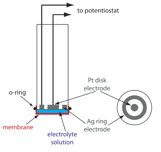
One important application of amperometry is in the construction of chemical sensors. One of the first amperometric sensors was developed in 1956 by L. C. Clark to measure dissolved O₂ in blood. Figure \(\PageIndex{9}\) shows the sensor’s design, which is similar to a potentiometric membrane electrode. A thin, gas-permeable membrane is stretched across the end of the sensor and is separated from the working electrode and the counter electrode by a thin solution of KCl. The working electrode is a Pt disk cathode, and a Ag ring anode serves as the counter electrode. Although several gases can diffuse across the membrane, including O₂, N₂, and CO₂, only oxygen undergoes reduction at the cathode

\[\mathrm{O}_{2}(g)+4 \mathrm{H}_{3} \mathrm{O}^{+}(a q)+4 e^{-}\rightleftharpoons 6 \mathrm{H}_{2} \mathrm{O}(l) \label{lsv17} \]

with its concentration at the electrode’s surface quickly reaching zero. The concentration of O₂ at the membrane’s inner surface is fixed by its diffusion through the membrane, which creates a limiting current. The result is a steady-state current that is proportional to the concentration of dissolved oxygen. Because the electrode consumes oxygen, the sample is stirred to prevent the depletion of O₂ at the membrane’s outer surface.

The oxidation of the Ag anode is the other half-reaction.

\[\mathrm{Ag}(s)+\text{ Cl}^{-}(a q)\rightleftharpoons \mathrm{AgCl}(s)+e^{-} \nonumber \]

Figure \(\PageIndex{9}\). Clark amperometric sensor for determining dissolved O₂. The diagram on the right is a cross-section through the electrode, which shows the Ag ring electrode and the Pt disk electrode.

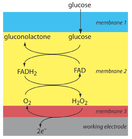
Another example of an amperometric sensor is a glucose sensor. In this sensor the single membrane in Figure \(\PageIndex{10}\) is replaced with three membranes. The outermost membrane of polycarbonate is permeable to glucose and O₂. The second membrane contains an immobilized preparation of glucose oxidase that catalyzes the oxidation of glucose to gluconolactone and hydrogen peroxide.

\[\beta-\mathrm{D}-\text {glucose }(a q)+\text{ O}_{2}(a q)+\mathrm{H}_{2} \mathrm{O}(l)\rightleftharpoons \text {gluconolactone }(a q)+\text{ H}_{2} \mathrm{O}_{2}(a q) \label{lsv18} \]

The hydrogen peroxide diffuses through the innermost membrane of cellulose acetate where it undergoes oxidation at a Pt anode.

\[\mathrm{H}_{2} \mathrm{O}_{2}(a q)+2 \mathrm{OH}^{-}(a q) \rightleftharpoons \text{ O}_{2}(a q)+2 \mathrm{H}_{2} \mathrm{O}(l)+2 e^{-} \label{lsv19} \]

Figure \(\PageIndex{10}\) summarizes the reactions that take place in this amperometric sensor. FAD is the oxidized form of flavin adenine nucleotide—the active site of the enzyme glucose oxidase—and FADH₂ is the active site’s reduced form. Note that O₂ serves a mediator, carrying electrons to the electrode.

Figure \(\PageIndex{10}\). Schematic showing the reactions by which an amperometric biosensor responds to glucose.

By changing the enzyme and mediator, it is easy to extend to the amperometric sensor in Figure \(\PageIndex{10}\) to the analysis of other analytes. For example, a CO₂ sensor has been developed using an amperometric O₂ sensor with a two-layer membrane, one of which contains an immobilized preparation of autotrophic bacteria [Karube, I.; Nomura, Y.; Arikawa, Y. Trends in Anal. Chem. 1995, 14, 295–299]. As CO₂ diffuses through the membranes it is converted to O₂ by the bacteria, increasing the concentration of O₂ at the Pt cathode.