14.3: Qualitative and Characterization Applications

Qualitative Applications

As discussed in Chapter 14.2, ultraviolet, visible, and infrared absorption bands result from the absorption of electromagnetic radiation by specific valence electrons or bonds. The energy at which the absorption occurs, and the intensity of that absorption, is determined by the chemical environment of the absorbing moiety. For example, benzene has several ultraviolet absorption bands due to \(\pi \rightarrow \pi^*\) transitions. The position and intensity of two of these bands, 203.5 nm (\(\epsilon\) = 7400 M^–1cm^–1) and 254 nm (\(\epsilon\) = 204 M^–1 cm^–1), are sensitive to substitution. For benzoic acid, in which a carboxylic acid group replaces one of the aromatic hydrogens, the two bands shift to 230 nm (\(\epsilon\) = 11600 M^–1 cm^–1) and 273 nm (\(\epsilon\) = 970 M^–1 cm^–1). A variety of rules have been developed to aid in correlating UV/Vis absorption bands to chemical structure. With the availability of computerized data acquisition and storage it is possible to build digital libraries of standard reference spectra. The identity of an a unknown compound often can be determined by comparing its spectrum against a library of reference spectra, a process known as spectral searching.

Characterization Applications

Molecular absorption, particularly in the UV/Vis range, has been used for a variety of different characterization studies, including determining the stoichiometry of metal–ligand complexes and determining equilibrium constants. Both of these examples are examined in this section.

Stoichiometry of a Metal-Ligand Complex

We can determine the stoichiometry of the metal–ligand complexation reaction

\[\mathrm{M}+y \mathrm{L} \rightleftharpoons \mathrm{ML}_{y} \nonumber \]

using one of three methods: the method of continuous variations, the mole-ratio method, and the slope-ratio method. Of these approaches, the method of continuous variations, also called Job’s method, is the most popular. In this method a series of solutions is prepared such that the total moles of metal and of ligand, n_total, in each solution is the same. If (n_M)_i and (n_L)_i are, respectively, the moles of metal and ligand in solution i, then

\[n_{\text { total }}=\ \left(n_{\mathrm{M}}\right)_{i} \ + \ \left(n_{\mathrm{L}}\right)_{i} \nonumber \]

The relative amount of ligand and metal in each solution is expressed as the mole fraction of ligand, (X_L)_i, and the mole fraction of metal, (X_M)_i,

\[\left(X_{\mathrm{L}}\right)_{i}=\frac{\left(n_{\mathrm{L}}\right)_{i}}{n_{\mathrm{total}}} \nonumber \]

\[\left(X_{M}\right)_{i}=1-\frac{\left(n_\text{L}\right)_{i}}{n_{\text { total }}}=\frac{\left(n_\text{M}\right)_{i}}{n_{\text { total }}} \nonumber \]

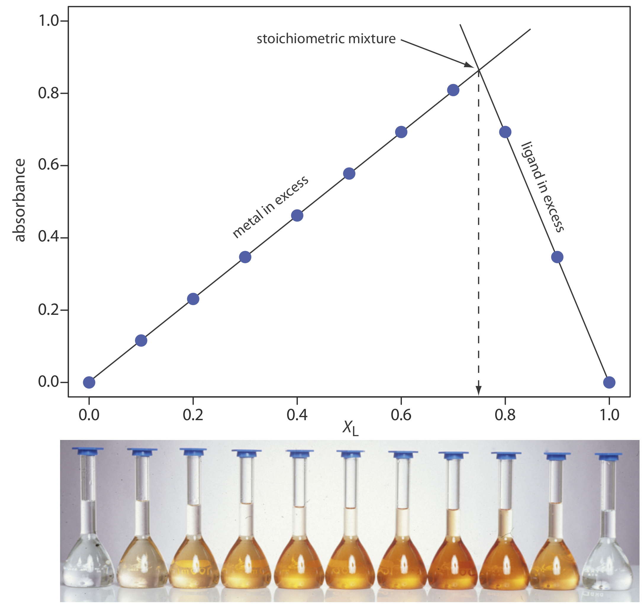
The concentration of the metal–ligand complex in any solution is determined by the limiting reagent, with the greatest concentration occurring when the metal and the ligand are mixed stoichiometrically. If we monitor the complexation reaction at a wavelength where only the metal–ligand complex absorbs, a graph of absorbance versus the mole fraction of ligand has two linear branches—one when the ligand is the limiting reagent and a second when the metal is the limiting reagent. The intersection of the two branches represents a stoichiometric mixing of the metal and the ligand. We use the mole fraction of ligand at the intersection to determine the value of y for the metal–ligand complex ML_y.

\[y=\frac{n_{\mathrm{L}}}{n_{\mathrm{M}}}=\frac{X_{\mathrm{L}}}{X_{\mathrm{M}}}=\frac{X_{\mathrm{L}}}{1-X_{\mathrm{L}}} \nonumber \]

You also can plot the data as absorbance versus the mole fraction of metal. In this case, y is equal to (1 – X_M)/X_M.

Example 14.3.1

To determine the formula for the complex between Fe²⁺ and o-phenanthroline, a series of solutions is prepared in which the total concentration of metal and ligand is held constant at \(3.15 \times 10^{-4}\) M. The absorbance of each solution is measured at a wavelength of 510 nm. Using the following data, determine the formula for the complex.

XL	absorbance	XL	absorbance
0.000	0.000	0.600	0.693
0.100	0.116	0.700	0.809
0.200	0.231	0.800	0.693
0.300	0.347	0.900	0.347
0.400	0.462	1.000	0.000
0.500	0.578

Solution

A plot of absorbance versus the mole fraction of ligand is shown in Figure \(\PageIndex{1}\). To find the maximum absorbance, we extrapolate the two linear portions of the plot. The two lines intersect at a mole fraction of ligand of 0.75. Solving for y gives

\[y=\frac{X_{L}}{1-X_{L}}=\frac{0.75}{1-0.75}=3 \nonumber \]

The formula for the metal–ligand complex is \(\text{Fe(phen)}_3^{2+}\).

Figure \(\PageIndex{1}\). Continuous variations plot for Example 14.3.1 . The photo shows the solutions used to gather the data. Each solution is displayed directly below its corresponding point on the continuous variations plot. To prepare these solutions I first prepared a solution of \(3.15 \times10^{-4}\) M Fe²⁺ and a solution of \(3.15 \times 10^{-4}\) M o-phenanthroline. Because the two stock solutions have the same concentration, diluting a portion of one solution with the other solution gives a mixture in which the combined concentration of o-phenanthroline and Fe²⁺ is \(3.15 \times 10^{-4}\) M. Because each solution has the same volume, each solution also contains the same total moles of metal and ligand.

Exercise 14.3.1

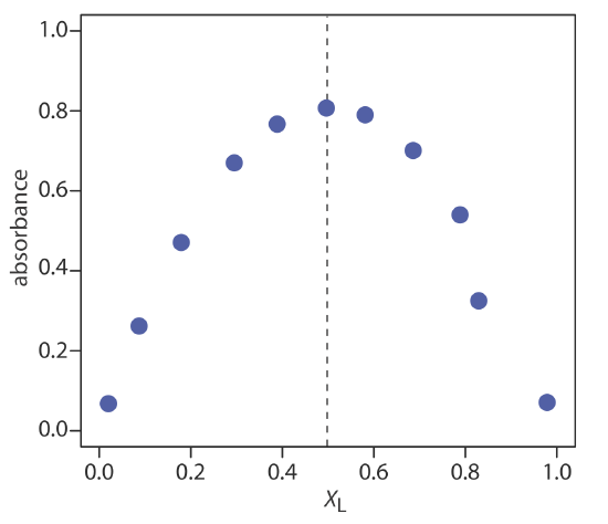
Use the continuous variations data in the following table to determine the formula for the complex between Fe²⁺ and SCN^–. The data for this problem is adapted from Meloun, M.; Havel, J.; Högfeldt, E. Computation of Solution Equilibria, Ellis Horwood: Chichester, England, 1988, p. 236.

XL	absorbance	XL	absorbance	XL	absorbance	XL	absorbance
0.0200	0.068	0.2951	0.670	0.5811	0.790	0.8923	0.324
0.0870	0.262	0.3887	0.767	0.6860	0.701	0.9787	0.071
0.1792	0.471	0.4964	0.807	0.7885	0.540

Answer

The figure below shows a continuous variations plot for the data in this exercise. Although the individual data points show substantial curvature—enough curvature that there is little point in trying to draw linear branches for excess metal and excess ligand—the maximum absorbance clearly occurs at X_L ≈ 0.5. The complex’s stoichiometry, therefore, is Fe(SCN)²⁺.

Several precautions are necessary when using the method of continuous variations. First, the metal and the ligand must form only one metal–ligand complex. To determine if this condition is true, plots of absorbance versus X_L are constructed at several different wavelengths and for several different values of n_total. If the maximum absorbance does not occur at the same value of X_L for each set of conditions, then more than one metal–ligand complex is present. A second precaution is that the metal–ligand complex’s absorbance must obey Beer’s law. Third, if the metal–ligand complex’s formation constant is relatively small, a plot of absorbance versus X_L may show significant curvature. In this case it often is difficult to determine the stoichiometry by extrapolation. Finally, because the stability of a metal–ligand complex may be influenced by solution conditions, it is necessary to control carefully the composition of the solutions. When the ligand is a weak base, for example, each solutions must be buffered to the same pH.

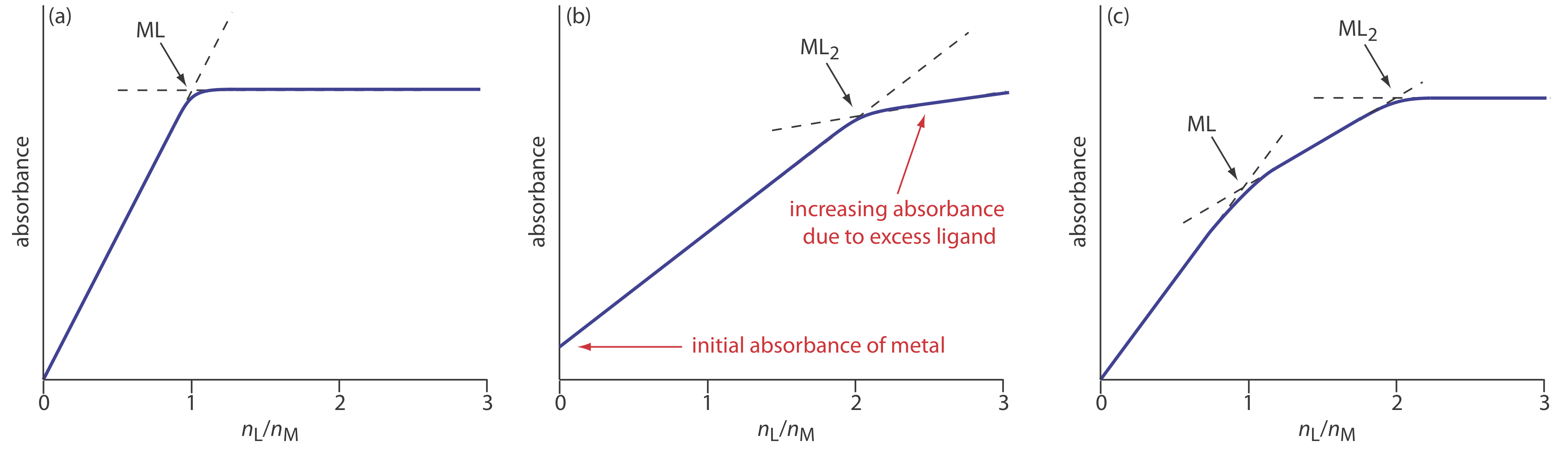
In the mole-ratio method the moles of one reactant, usually the metal, is held constant, while the moles of the other reactant is varied. The absorbance is monitored at a wavelength where the metal–ligand complex absorbs. A plot of absorbance as a function of the ligand-to-metal mole ratio, n_L/n_M, has two linear branches that intersect at a mole–ratio corresponding to the complex’s formula. Figure \(\PageIndex{2}a\) shows a mole-ratio plot for the formation of a 1:1 complex in which the absorbance is monitored at a wavelength where only the complex absorbs. Figure \(\PageIndex{2}b\) shows a mole-ratio plot for a 1:2 complex in which all three species—the metal, the ligand, and the complex—absorb at the selected wavelength. Unlike the method of continuous variations, the mole-ratio method can be used for complexation reactions that occur in a stepwise fashion if there is a difference in the molar absorptivities of the metal–ligand complexes, and if the formation constants are sufficiently different. A typical mole-ratio plot for the step-wise formation of ML and ML₂ is shown in Figure \(\PageIndex{2}c\).

Figure \(\PageIndex{2}a\). Mole-ratio plots for: (a) a 1:1 metal–ligand complex in which only the complex absorbs; (b) a 1:2 metal–ligand complex in which the metal, the ligand, and the complex absorb; and (c) the stepwise formation of a 1:1 and a 1:2 metal–ligand complex.

For both the method of continuous variations and the mole-ratio method, we determine the complex’s stoichiometry by extrapolating absorbance data from conditions in which there is a linear relationship between absorbance and the relative amounts of metal and ligand. If a metal–ligand complex is very weak, a plot of absorbance versus X_L or n_L/n_M becomes so curved that it is impossible to determine the stoichiometry by extrapolation. In this case the slope-ratio is used.

In the slope-ratio method two sets of solutions are prepared. The first set of solutions contains a constant amount of metal and a variable amount of ligand, chosen such that the total concentration of metal, C_M, is much larger than the total concentration of ligand, C_L. Under these conditions we may assume that essentially all the ligand reacts to form the metal–ligand complex. The concentration of the complex, which has the general form M_xL_y, is

\[\left[\mathrm{M}_{x} \mathrm{L_y}\right]=\frac{C_{\mathrm{L}}}{y} \nonumber \]

If we monitor the absorbance at a wavelength where only M_xL_y absorbs, then

\[A=\varepsilon b\left[\mathrm{M}_{x} \mathrm{L}_{y}\right]=\frac{\varepsilon b C_{\mathrm{L}}}{y} \nonumber \]

and a plot of absorbance versus C_L is linear with a slope, s_L, of

\[s_{\mathrm{L}}=\frac{\varepsilon b}{y}\ ]

A second set of solutions is prepared with a fixed concentration of ligand that is much greater than a variable concentration of metal; thus

\[\left[\mathrm{M}_{x} \mathrm{L}_{y}\right]=\frac{C_{\mathrm{M}}}{x} \nonumber \]

\[A=\varepsilon b\left[\mathrm{M}_{x} \mathrm{L}_{y}\right]=\frac{\varepsilon b C_{\mathrm{M}}}{x} \nonumber \]

\[s_{M}=\frac{\varepsilon b}{x} \nonumber \]

A ratio of the slopes provides the relative values of x and y.

\[\frac{s_{\text{M}}}{s_{\text{L}}}=\frac{\varepsilon b / x}{\varepsilon b / y}=\frac{y}{x} \nonumber \]

An important assumption in the slope-ratio method is that the complexation reaction continues to completion in the presence of a sufficiently large excess of metal or ligand. The slope-ratio method also is limited to systems in which only a single complex forms and for which Beer’s law is obeyed.

Determination of Equilibrium Constants

Another important application of molecular absorption spectroscopy is the determination of equilibrium constants. Let’s consider, as a simple example, an acid–base reaction of the general form

\[\operatorname{HIn}(a q)+ \ \mathrm{H}_{2} \mathrm{O}(l) \rightleftharpoons \ \mathrm{H}_{3} \mathrm{O}^{+}(a q)+\operatorname{In}^{-}(a q) \nonumber \]

where HIn and In^– are the conjugate weak acid and weak base forms of an acid–base indicator. The equilibrium constant for this reaction is

\[K_{\mathrm{a}}=\frac{\left[\mathrm{H}_{3} \mathrm{O}^{+}\right][\mathrm{A^-}]}{[\mathrm{HA}]} \nonumber \]

To determine the equilibrium constant’s value, we prepare a solution in which the reaction is in a state of equilibrium and determine the equilibrium concentration for H₃O⁺, HIn, and In^–. The concentration of H₃O⁺ is easy to determine by measuring the solution’s pH. To determine the concentration of HIn and In^– we can measure the solution’s absorbance.

If both HIn and In^– absorb at the selected wavelength, then, from Beer's law, we know that

\[A=\varepsilon_{\mathrm{Hln}} b[\mathrm{HIn}]+\varepsilon_{\mathrm{ln}} b[\mathrm{In}^-] \label{10.5} \]

where \(\varepsilon_\text{HIn}\) and \(\varepsilon_{\text{In}}\) are the molar absorptivities for HIn and In^–. The indicator’s total concentration, C, is given by a mass balance equation

\[C=[\mathrm{HIn}]+ [\text{In}^-] \label{10.6} \]

Solving Equation \ref{10.6} for [HIn] and substituting into Equation \ref{10.5} gives

\[A=\varepsilon_{\mathrm{Hln}} b\left(C-\left[\mathrm{In}^{-}\right]\right)+\varepsilon_{\mathrm{ln}} b\left[\mathrm{In}^{-}\right] \nonumber \]

which we simplify to

\[A=\varepsilon_{\mathrm{Hln}} bC- \varepsilon_{\mathrm{Hln}}b\left[\mathrm{In}^{-}\right]+\varepsilon_{\mathrm{ln}} b\left[\mathrm{In}^{-}\right] \nonumber \]

\[A=A_{\mathrm{HIn}}+b\left[\operatorname{In}^{-}\right]\left(\varepsilon_{\mathrm{ln}}-\varepsilon_{\mathrm{HIn}}\right) \label{10.7} \]

where A_HIn, which is equal to \(\varepsilon_\text{HIn}bC\), is the absorbance when the pH is acidic enough that essentially all the indicator is present as HIn. Solving Equation \ref{10.7} for the concentration of In^– gives

\[\left[\operatorname{In}^{-}\right]=\frac{A-A_{\mathrm{Hln}}}{b\left(\varepsilon_{\mathrm{ln}}-\varepsilon_{\mathrm{HIn}}\right)} \label{10.8} \]

Proceeding in the same fashion, we derive a similar equation for the concentration of HIn

\[[\mathrm{HIn}]=\frac{A_{\mathrm{In}}-A}{b\left(\varepsilon_{\mathrm{ln}}-\varepsilon_{\mathrm{Hln}}\right)} \label{10.9} \]

where A_In, which is equal to \(\varepsilon_{\text{In}}bC\), is the absorbance when the pH is basic enough that only In^– contributes to the absorbance. Substituting Equation \ref{10.8} and Equation \ref{10.9} into the equilibrium constant expression for HIn gives

\[K_a = \frac {[\text{H}_3\text{O}^+][\text{In}^-]} {[\text{HIn}]} = [\text{H}_3\text{O}^+] \times \frac {A - A_\text{HIn}} {A_{\text{In}} - A} \label{10.10} \]

We can use Equation \ref{10.10} to determine K_a in one of two ways. The simplest approach is to prepare three solutions, each of which contains the same amount, C, of indicator. The pH of one solution is made sufficiently acidic such that [HIn] >> [In^–]. The absorbance of this solution gives A_HIn. The value of A_In is determined by adjusting the pH of the second solution such that [In^–] >> [HIn]. Finally, the pH of the third solution is adjusted to an intermediate value, and the pH and absorbance, A, recorded. The value of K_a is calculated using Equation \ref{10.10}.

Example 14.3.2

The acidity constant for an acid–base indicator is determined by preparing three solutions, each of which has a total concentration of indicator equal to \(5.00 \times 10^{-5}\) M. The first solution is made strongly acidic with HCl and has an absorbance of 0.250. The second solution is made strongly basic and has an absorbance of 1.40. The pH of the third solution is 2.91 and has an absorbance of 0.662. What is the value of K_a for the indicator?

Solution

The value of K_a is determined by making appropriate substitutions into 10.20 where [H₃O⁺] is \(1.23 \times 10^{-3}\); thus

\[K_{\mathrm{a}}=\left(1.23 \times 10^{-3}\right) \times \frac{0.662-0.250}{1.40-0.662}=6.87 \times 10^{-4} \nonumber \]

Exercise 14.3.2

To determine the K_a of a merocyanine dye, the absorbance of a solution of \(3.5 \times 10^{-4}\) M dye was measured at a pH of 2.00, a pH of 6.00, and a pH of 12.00, yielding absorbances of 0.000, 0.225, and 0.680, respectively. What is the value of K_a for this dye? The data for this problem is adapted from Lu, H.; Rutan, S. C. Anal. Chem., 1996, 68, 1381–1386.

Answer

The value of K_a is

\[K_{\mathrm{a}}=\left(1.00 \times 10^{-6}\right) \times \frac{0.225-0.000}{0.680-0.225}=4.95 \times 10^{-7} \nonumber \]

A second approach for determining K_a is to prepare a series of solutions, each of which contains the same amount of indicator. Two solutions are used to determine values for A_HIn and A_In. Taking the log of both sides of Equation \ref{10.10} and rearranging leave us with the following equation.

\[\log \frac{A-A_{\mathrm{Hin}}}{A_{\mathrm{ln}^{-}}-A}=\mathrm{pH}-\mathrm{p} K_{\mathrm{a}} \label{10.11} \]

A plot of log[(A – A_HIn)/(A_In – A)] versus pH is a straight-line with a slope of +1 and a y-intercept of –pK_a.

Exercise 14.3.3

To determine the K_a for the indicator bromothymol blue, the absorbance of each a series of solutions that contain the same concentration of bromothymol blue is measured at pH levels of 3.35, 3.65, 3.94, 4.30, and 4.64, yielding absorbance values of 0.170, 0.287, 0.411, 0.562, and 0.670, respectively. Acidifying the first solution to a pH of 2 changes its absorbance to 0.006, and adjusting the pH of the last solution to 12 changes its absorbance to 0.818. What is the value of K_a for bromothymol blue? The data for this problem is from Patterson, G. S. J. Chem. Educ., 1999, 76, 395–398.

Answer

To determine K_a we use Equation \ref{10.11}, plotting log[(A – A_HIn)/(A_In – A)] versus pH, as shown below.

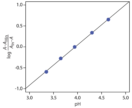
Fitting a straight-line to the data gives a regression model of

\[\log \frac{A-A_{\mathrm{HIn}}}{A_{\mathrm{ln}}-A}=-3.80+0.962 \mathrm{pH} \nonumber \]

The y-intercept is –pK_a; thus, the pK_a is 3.80 and the K_a is \(1.58 \times 10^{-4}\).

In developing these approaches for determining K_a we considered a relatively simple system in which the absorbance of HIn and In^– are easy to measure and for which it is easy to determine the concentration of H₃O⁺. In addition to acid–base reactions, we can adapt these approaches to any reaction of the general form

\[X(a q)+Y(a q)\rightleftharpoons Z(a q) \nonumber \]

including metal–ligand complexation reactions and redox reactions, provided we can determine spectrophotometrically the concentration of the product, Z, and one of the reactants, either X or Y, and that we can determine the concentration of the other reactant by some other method. With appropriate modifications, a more complicated system in which we cannot determine the concentration of one or more of the reactants or products also is possible [Ramette, R. W. Chemical Equilibrium and Analysis, Addison-Wesley: Reading, MA, 1981, Chapter 13].