14.4: Quantitative Applications

Scope

The determination of an analyte’s concentration based on its absorption of ultraviolet or visible radiation is one of the most frequently encountered quantitative analytical methods. One reason for its popularity is that many organic and inorganic compounds have strong absorption bands in the UV/Vis region of the electromagnetic spectrum. In addition, if an analyte does not absorb UV/Vis radiation—or if its absorbance is too weak—we often can react it with another species that is strongly absorbing. For example, a dilute solution of Fe²⁺ does not absorb visible light. Reacting Fe²⁺ with o-phenanthroline, however, forms an orange–red complex of \(\text{Fe(phen)}_3^{2+}\) that has a strong, broad absorbance band near 500 nm. An additional advantage to UV/Vis absorption is that in most cases it is relatively easy to adjust experimental and instrumental conditions so that Beer’s law is obeyed.

Environmental Applications

The analysis of waters and wastewaters often relies on the absorption of ultraviolet and visible radiation. Many of these methods are outlined in Table \(\PageIndex{1}\). Several of these methods are described here in more detail.

Table \(\PageIndex{1}\). Examples of Molecular UV/Vis Analysis of Waters and Wastewaters

analyte	method	\(\lambda\) (nm)
trace metals
aluminum	react with Eriochrome cyanide R dye at pH 6; forms red to pink complex	535
arsenic	reduce to AsH3 using Zn and react with silver diethyldithiocarbamate; forms red complex	535
cadmium	extract into CHCl3 containing dithizone from a sample made basic with NaOH; forms pink to red complex	518
chromium	oxidize to Cr(VI) and react with diphenylcarbazide; forms 540 red-violet product	540
copper	react with neocuprine in neutral to slightly acid solution and extract into CHCl3/CH3OH; forms yellow complex	457
iron	reduce to Fe^2^+ and react with o-phenanthroline; forms orange-red complex	510
lead	extract into CHCl3 containing dithizone from sample made basic with NH3/ NH4^+ buffer; forms cherry red complex	510
manganese	oxidize to MnO4^– with persulfate; forms purple solution	525
mercury	extract into CHCl3 containing dithizone from acidic sample; forms orange complex	492
zinc	react with zincon at pH 9; forms blue complex	620
inorganic nonmetals
ammonia	reaction with hypochlorite and phenol using a manganous 630 salt catalyst; forms blue indophenol as product	630
cyanide	react with chloroamine-T to form CNCl and then with a pyridine-barbituric acid; forms a red-blue dye	578
fluoride	react with red Zr-SPADNS lake; formation of ZrF6^2^–decreases color of the red lake	570
chlorine (residual)	react with leuco crystal violet; forms blue product	592
nitrate	react with Cd to form NO2^– and then react with sulfanilamide and N-(1-napthyl)-ethylenediamine; forms red azo 543 dye	543
phosphate	react with ammonium molybdate and then reduce with SnCl2; forms molybdenum blue	690
organics
phenol	react with 4-aminoantipyrine and K3Fe(CN)6; forms yellow antipyrine dye	460
anionic surfactants	react with cationic methylene blue dye and extract into CHCl3; forms blue ion pair	652

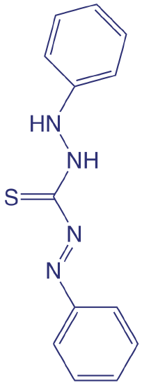
Although the quantitative analysis of metals in waters and wastewaters is accomplished primarily by atomic absorption or atomic emission spectroscopy, many metals also can be analyzed following the formation of a colorful metal–ligand complex. One advantage to these spectroscopic methods is that they easily are adapted to the analysis of samples in the field using a filter photometer. One ligand used for the analysis of several metals is diphenylthiocarbazone, also known as dithizone. Dithizone is not soluble in water, but when a solution of dithizone in CHCl₃ is shaken with an aqueous solution that contains an appropriate metal ion, a colored metal–dithizonate complex forms that is soluble in CHCl₃. The selectivity of dithizone is controlled by adjusting the sample’s pH. For example, Cd²⁺ is extracted from solutions made strongly basic with NaOH, Pb²⁺ from solutions made basic with an NH₃/ NH₄⁺ buffer, and Hg²⁺ from solutions that are slightly acidic.

The structure of dithizone is shown below.

When chlorine is added to water the portion available for disinfection is called the chlorine residual. There are two forms of chlorine residual. The free chlorine residual includes Cl₂, HOCl, and OCl^–. The combined chlorine residual, which forms from the reaction of NH₃ with HOCl, consists of monochloramine, NH₂Cl, dichloramine, NHCl₂, and trichloramine, NCl₃. Because the free chlorine residual is more efficient as a disinfectant, there is an interest in methods that can distinguish between the total chlorine residual’s different forms. One such method is the leuco crystal violet method. The free residual chlorine is determined by adding leuco crystal violet to the sample, which instantaneously oxidizes to give a blue-colored compound that is monitored at 592 nm. Completing the analysis in less than five minutes prevents a possible interference from the combined chlorine residual. The total chlorine residual (free + combined) is determined by reacting a separate sample with iodide, which reacts with both chlorine residuals to form HOI. When the reaction is complete, leuco crystal violet is added and oxidized by HOI, giving the same blue-colored product. The combined chlorine residual is determined by difference.

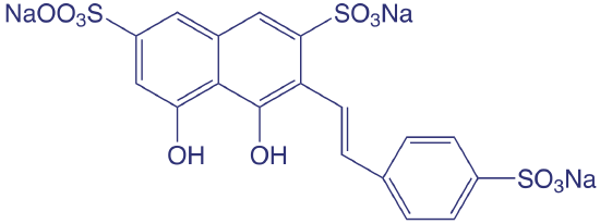
The concentration of fluoride in drinking water is determined indirectly by its ability to form a complex with zirconium. In the presence of the dye SPADNS, a solution of zirconium forms a red colored compound, called a lake, that absorbs at 570 nm. When fluoride is added, the formation of the stable \(\text{ZrF}_6^{2-}\) complex causes a portion of the lake to dissociate, decreasing the absorbance. A plot of absorbance versus the concentration of fluoride, therefore, has a negative slope.

SPADNS, the structure of which is shown below, is an abbreviation for the sodium salt of 2-(4-sulfophenylazo)-1,8-dihydroxy-3,6-napthalenedisulfonic acid, which is a mouthful to say.

Spectroscopic methods also are used to determine organic constituents in water. For example, the combined concentrations of phenol and ortho- and meta-substituted phenols are determined by using steam distillation to separate the phenols from nonvolatile impurities. The distillate reacts with 4-aminoantipyrine at pH 7.9 ± 0.1 in the presence of K₃Fe(CN)₆ to a yellow colored antipyrine dye. After extracting the dye into CHCl₃, its absorbance is monitored at 460 nm. A calibration curve is prepared using only the unsubstituted phenol, C₆H₅OH. Because the molar absorptivity of substituted phenols generally are less than that for phenol, the reported concentration represents the minimum concentration of phenolic compounds.

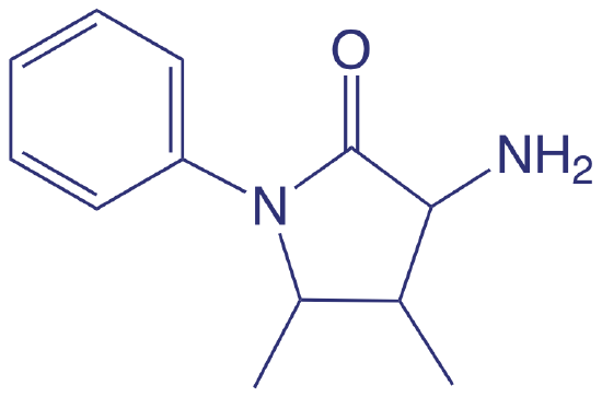
4-aminoantipyrene

Molecular absorption also is used for the analysis of environmentally significant airborne pollutants. In many cases the analysis is carried out by collecting the sample in water, converting the analyte to an aqueous form that can be analyzed by methods such as those described in Table \(\PageIndex{1}\). For example, the concentration of NO₂ is determined by oxidizing NO₂ to \(\text{NO}_3^-\). The concentration of \(\text{NO}_3^-\) is then determined by first reducing it to \(\text{NO}_2^-\) with Cd, and then reacting \(\text{NO}_2^-\) with sulfanilamide and N-(1-naphthyl)-ethylenediamine to form a red azo dye. Another important application is the analysis for SO₂, which is determined by collecting the sample in an aqueous solution of \(\text{HgCl}_4^{2-}\) where it reacts to form \(\text{Hg(SO}_3)_2^{2-}\). Addition of p-rosaniline and formaldehyde produces a purple complex that is monitored at 569 nm. Infrared absorption is useful for the analysis of organic vapors, including HCN, SO₂, nitrobenzene, methyl mercaptan, and vinyl chloride. Frequently, these analyses are accomplished using portable, dedicated infrared photometers.

Clinical Applications

The analysis of clinical samples often is complicated by the complexity of the sample’s matrix, which may contribute a significant background absorption at the desired wavelength. The determination of serum barbiturates provides one example of how this problem is overcome. The barbiturates are first extracted from a sample of serum with CHCl₃ and then extracted from the CHCl₃ into 0.45 M NaOH (pH ≈ 13). The absorbance of the aqueous extract is measured at 260 nm, and includes contributions from the barbiturates as well as other components extracted from the serum sample. The pH of the sample is then lowered to approximately 10 by adding NH₄Cl and the absorbance remeasured. Because the barbiturates do not absorb at this pH, we can use the absorbance at pH 10, A_{pH 10}, to correct the absor-ance at pH 13, A_{pH 13}

\[A_\text{barb} = A_\text{pH 13} - \frac {V_\text{samp} + V_{\text{NH}_4\text{Cl}}} {V_\text{samp}} \times A_\text{pH 10} \nonumber \]

where A_barb is the absorbance due to the serum barbiturates and V_samp and \(V_{\text{NH}_4\text{Cl}}\) are the volumes of sample and NH₄Cl, respectively. Table \(\PageIndex{2}\) provides a summary of several other methods for analyzing clinical samples.

Table \(\PageIndex{2}\). Examples of the Molecular UV/Vis Analysis of Clinical Samples

analyte	method	\(\lambda\) (nm)
total serum protein	react with NaOH and Cu^2^+; forms blue-violet complex	540
serum cholesterol	react with Fe^3^+ in presence of isopropanol, acetic acid, and H2SO4; forms blue-violet complex	540
uric acid	react with phosphotungstic acid; forms tungsten blue	710
serum barbituates	extract into CHCl3 to isolate from interferents and then extract into 0.45 M NaOH	260
glucose	react with o-toludine at 100^oC; forms blue-green complex	630
protein-bound iodine	decompose protein to release iodide, which catalyzes redox reaction between Ce^3^+ and As^3^+; forms yellow colored Ce^4^+	420

Industrial Applications

UV/Vis molecular absorption is used for the analysis of a diverse array of industrial samples including pharmaceuticals, food, paint, glass, and metals. In many cases the methods are similar to those described in Table \(\PageIndex{1}\) and in Table \(\PageIndex{2}\). For example, the amount of iron in food is determined by bringing the iron into solution and analyzing using the o-phenanthroline method listed in Table \(\PageIndex{1}\).

Many pharmaceutical compounds contain chromophores that make them suitable for analysis by UV/Vis absorption. Products analyzed in this fashion include antibiotics, hormones, vitamins, and analgesics. One example of the use of UV absorption is in determining the purity of aspirin tablets, for which the active ingredient is acetylsalicylic acid. Salicylic acid, which is produced by the hydrolysis of acetylsalicylic acid, is an undesirable impurity in aspirin tablets, and should not be present at more than 0.01% w/w. Samples are screened for unacceptable levels of salicylic acid by monitoring the absorbance at a wavelength of 312 nm. Acetylsalicylic acid absorbs at 280 nm, but absorbs poorly at 312 nm. Conditions for preparing the sample are chosen such that an absorbance of greater than 0.02 signifies an unacceptable level of salicylic acid.

Forensic Applications

UV/Vis molecular absorption routinely is used for the analysis of narcotics and for drug testing. One interesting forensic application is the determination of blood alcohol using the Breathalyzer test. In this test a 52.5-mL breath sample is bubbled through an acidified solution of K₂Cr₂O₇, which oxidizes ethanol to acetic acid. The concentration of ethanol in the breath sample is determined by a decrease in the absorbance at 440 nm where the dichromate ion absorbs. A blood alcohol content of 0.10%, which is above the legal limit, corresponds to 0.025 mg of ethanol in the breath sample.

Developing a Quantitative Method for a Single Component

To develop a quantitative analytical method, the conditions under which Beer’s law is obeyed must be established. First, the most appropriate wavelength for the analysis is determined from an absorption spectrum. In most cases the best wavelength corresponds to an absorption maximum because it provides greater sensitivity and is less susceptible to instrumental limitations. Second, if the instrument has adjustable slits, then an appropriate slit width is chosen. The absorption spectrum also aids in selecting a slit width by choosing a width that is narrow enough to avoid instrumental limitaions to Beer’s law, but wide enough to increase the throughput of source radiation. Finally, a calibration curve is constructed to determine the range of concentrations for which Beer’s law is valid. Additional considerations that are important in any quantitative method are the effect of potential interferents and establishing an appropriate blank.

Quantitative Analysis for a Single Sample

To determine the concentration of an analyte we measure its absorbance and apply Beer’s law using any of the standardization methods described in Chapter 5. The most common methods are a normal calibration curve using external standards and the method of standard additions. A single point standardization also is possible, although we must first verify that Beer’s law holds for the concentration of analyte in the samples and the standard.

Example 14.4.1

The determination of iron in an industrial waste stream is carried out by the o-phenanthroline described in Representative Method 10.3.1. Using the data in the following table, determine the mg Fe/L in the waste stream.

mg Fe/L	absorbance
0.00	0.000
1.00	0.183
2.00	0.364
3.00	0.546
4.00	0.727
sample	0.269

Solution

Linear regression of absorbance versus the concentration of Fe in the standards gives the calibration curve and calibration equation shown here

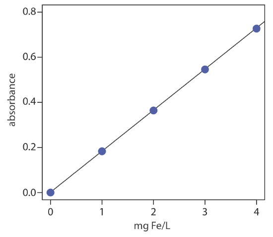
\[A=0.0006+\left(0.1817 \ \mathrm{mg}^{-1} \mathrm{L}\right) \times(\mathrm{mg} \mathrm{Fe} / \mathrm{L}) \nonumber \]

Substituting the sample’s absorbance into the calibration equation gives the concentration of Fe in the waste stream as 1.48 mg Fe/L

Exercise 14.4.1

The concentration of Cu²⁺ in a sample is determined by reacting it with the ligand cuprizone and measuring its absorbance at 606 nm in a 1.00-cm cell. When a 5.00-mL sample is treated with cuprizone and diluted to 10.00 mL, the resulting solution has an absorbance of 0.118. A second 5.00-mL sample is mixed with 1.00 mL of a 20.00 mg/L standard of Cu²⁺, treated with cuprizone and diluted to 10.00 mL, giving an absorbance of 0.162. Report the mg Cu²⁺/L in the sample.

Answer

For this standard addition we write equations that relate absorbance to the concentration of Cu²⁺ in the sample before the standard addition

\[0.118=\varepsilon b \left[ C_{\mathrm{Cu}} \times \frac{5.00 \text{ mL}}{10.00 \text{ mL}}\right] \nonumber \]

and after the standard addition

\[0.162=\varepsilon b\left(C_{\mathrm{Cu}} \times \frac{5.00 \text{ mL}}{10.00 \text{ mL}}+\frac{20.00 \ \mathrm{mg} \ \mathrm{Cu}}{\mathrm{L}} \times \frac{1.00 \ \mathrm{mL}}{10.00 \ \mathrm{mL}}\right) \nonumber \]

in each case accounting for the dilution of the original sample and for the standard. The value of \(\varepsilon b\) is the same in both equation. Solving each equation for \(\varepsilon b\) and equating

\[\frac{0.162}{C_{\mathrm{Cu}} \times \frac{5.00 \text{ mL}}{10.00 \text{ mL}}+\frac{20.00 \ \mathrm{mg} \ \mathrm{Cu}}{\mathrm{L}} \times \frac{1.00 \ \mathrm{mL}}{10.00 \ \mathrm{mL}}}=\frac{0.118}{C_{\mathrm{Cu}} \times \frac{5.00 \text{ mL}}{10.00 \text{ mL}}} \nonumber \]

leaves us with an equation in which C_Cu is the only variable. Solving for C_Cu gives its value as

\[\frac{0.162}{0.500 \times C_{\mathrm{Cu}}+2.00 \ \mathrm{mg} \ \mathrm{Cu} / \mathrm{L}}=\frac{0.118}{0.500 \times C_{\mathrm{Cu}}} \nonumber \]

\[0.0810 \times C_{\mathrm{Cu}}=0.0590 \times C_{\mathrm{Ca}}+0.236 \ \mathrm{mg} \ \mathrm{Cu} / \mathrm{L} \nonumber \]

\[0.0220 \times C_{\mathrm{Cu}}=0.236 \ \mathrm{mg} \ \mathrm{Cu} / \mathrm{L} \nonumber \]

\[C_{\mathrm{Cu}}=10.7 \ \mathrm{mg} \ \mathrm{Cu} / \mathrm{L} \nonumber \]

Quantitative Analysis of Mixtures

Suppose we need to determine the concentration of two analytes, X and Y, in a sample. If each analyte has a wavelength where the other analyte does not absorb, then we can proceed using the approach in Example 14.4.1 . Unfortunately, UV/Vis absorption bands are so broad that frequently it is not possible to find suitable wavelengths. Because Beer’s law is additive the mixture’s absorbance, A_mix, is

\[\left(A_{m i x}\right)_{\lambda_{1}}=\left(\varepsilon_{x}\right)_{\lambda_{1}} b C_{X}+\left(\varepsilon_{Y}\right)_{\lambda_{1}} b C_{Y} \label{10.1} \]

where \(\lambda_1\) is the wavelength at which we measure the absorbance. Because Equation \ref{10.1} includes terms for the concentration of both X and Y, the absorbance at one wavelength does not provide enough information to determine either C_X or C_Y. If we measure the absorbance at a second wavelength

\[\left(A_{m i x}\right)_{\lambda_{2}}=\left(\varepsilon_{x}\right)_{\lambda_{2}} b C_{X}+\left(\varepsilon_{Y}\right)_{\lambda_{2}} b C_{Y} \label{10.2} \]

then we can determine C_X and C_Y by solving simultaneously Equation \ref{10.1} and Equation \ref{10.2}. Of course, we also must determine the value for \(\varepsilon_X\) and \(\varepsilon_Y\) at each wavelength. For a mixture of n components, we must measure the absorbance at n different wavelengths.

Example 14.4.2

The concentrations of Fe³⁺ and Cu²⁺ in a mixture are determined following their reaction with hexacyanoruthenate (II), \(\text{Ru(CN)}_6^{4-}\), which forms a purple-blue complex with Fe³⁺ (\(\lambda_\text{max}\) = 550 nm) and a pale-green complex with Cu²⁺ (\(\lambda_\text{max}\) = 396 nm) [DiTusa, M. R.; Schlit, A. A. J. Chem. Educ. 1985, 62, 541–542]. The molar absorptivities (M^–1 cm^–1) for the metal complexes at the two wavelengths are summarized in the following table.

analyte	\(\varepsilon_{550}\)	\(\varepsilon_{396}\)
Fe^3^+	9970	84
Cu^2^+	34	856

When a sample that contains Fe³⁺ and Cu²⁺ is analyzed in a cell with a pathlength of 1.00 cm, the absorbance at 550 nm is 0.183 and the absorbance at 396 nm is 0.109. What are the molar concentrations of Fe³⁺ and Cu²⁺ in the sample?

Solution

Substituting known values into Equation \ref{10.1} and Equation \ref{10.2} gives

\[\begin{aligned} A_{550} &=0.183=9970 C_{\mathrm{Fe}}+34 C_{\mathrm{Cu}} \\ A_{396} &=0.109=84 C_{\mathrm{Fe}}+856 C_{\mathrm{Cu}} \end{aligned} \nonumber \]

To determine C_Fe and C_Cu we solve the first equation for C_Cu

\[C_{\mathrm{Cu}}=\frac{0.183-9970 C_{\mathrm{Fe}}}{34} \nonumber \]

and substitute the result into the second equation.

\[\begin{aligned} 0.109 &=84 C_{\mathrm{Fe}}+856 \times \frac{0.183-9970 C_{\mathrm{Fe}}}{34} \\ &=4.607-\left(2.51 \times 10^{5}\right) C_{\mathrm{Fe}} \end{aligned} \nonumber \]

Solving for C_Fe gives the concentration of Fe³⁺ as \(1.8 \times 10^{-5}\) M. Substituting this concentration back into the equation for the mixture’s absorbance at 396 nm gives the concentration of Cu²⁺ as \(1.3 \times 10^{-4}\) M.

Another approach to solving Example 14.4.2 is to multiply the first equation by 856/34 giving

\[4.607=251009 C_{\mathrm{Fe}}+856 C_\mathrm{Cu} \nonumber \]

Subtracting the second equation from this equation

\[\begin{aligned} 4.607 &=251009 C_{\mathrm{Fe}}+856 C_{\mathrm{Cu}} \\-0.109 &=84 C_{\mathrm{Fe}}+856 C_{\mathrm{Cu}} \end{aligned} \nonumber \]

gives

\[4.498=250925 C_{\mathrm{Fe}} \nonumber \]

and we find that C_Fe is \(1.8 \times 10^{-5}\). Having determined C_Fe we can substitute back into one of the other equations to solve for C_Cu, which is \(1.3 \times 10^{-5}\).

Exercise 14.4.2

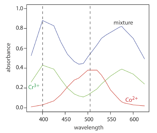
The absorbance spectra for Cr³⁺ and Co²⁺ overlap significantly. To determine the concentration of these analytes in a mixture, its absorbance is measured at 400 nm and at 505 nm, yielding values of 0.336 and 0.187, respectively. The individual molar absorptivities (M^–1 cm^–1) for Cr3⁺ are 15.2 at 400 nm and 0.533 at 505 nm; the values for Co²⁺ are 5.60 at 400 nm and 5.07 at 505 nm.

Answer

Substituting into Equation \ref{10.1} and Equation \ref{10.2} gives

\[A_{400} = 0.336 = 15.2C_\text{Cr} + 5.60C_\text{Co} \nonumber \]

\[A_{400} = 0187 = 0.533C_\text{Cr} + 5.07C_\text{Co} \nonumber \]

To determine C_Cr and C_Co we solve the first equation for C_Co

\[C_{\mathrm{Co}}=\frac{0.336-15.2 \mathrm{C}_{\mathrm{Co}}}{5.60} \nonumber \]

and substitute the result into the second equation.

\[0.187=0.533 C_{\mathrm{Cr}}+5.07 \times \frac{0.336-15.2 C_{\mathrm{Co}}}{5.60} \nonumber \]

\[0.187=0.3042-13.23 C_{\mathrm{Cr}} \nonumber \]

Solving for C_Cr gives the concentration of Cr³⁺ as \(8.86 \times 10^{-3}\) M. Substituting this concentration back into the equation for the mixture’s absorbance at 400 nm gives the concentration of Co²⁺ as \(3.60 \times 10^{-2}\) M.

To obtain results with good accuracy and precision the two wavelengths should be selected so that \(\varepsilon_X > \varepsilon_Y\) at one wavelength and \(\varepsilon_X < \varepsilon_Y\) at the other wavelength. It is easy to appreciate why this is true. Because the absorbance at each wavelength is dominated by one analyte, any uncertainty in the concentration of the other analyte has less of an impact. Figure \(\PageIndex{q}\) shows that the choice of wavelengths for Practice Exercise 14.4.2 are reasonable. When the choice of wavelengths is not obvious, one method for locating the optimum wavelengths is to plot \(\varepsilon_X / \varepsilon_y\) as function of wavelength, and determine the wavelengths where \(\varepsilon_X / \varepsilon_y\) reaches maximum and minimum values [Mehra, M. C.; Rioux, J. J. Chem. Educ. 1982, 59, 688–689].

Figure \(\PageIndex{1}\). Visible absorption spectra for 0.0250 M Cr³⁺, 0.0750 M Co²⁺, and for a mixture of Cr³⁺ and Co²⁺. The two wavelengths used to analyze the mixture of Cr³⁺ and Co²⁺ are shown by the dashed lines. The data for the two standards are from Brewer, S. Solving Problems in Analytical Chemistry, John Wiley & Sons: New York, 1980.

When the analyte’s spectra overlap severely, such that \(\varepsilon_X \approx \varepsilon_Y\) at all wavelengths, other computational methods may provide better accuracy and precision. In a multiwavelength linear regression analysis, for example, a mixture’s absorbance is compared to that for a set of standard solutions at several wavelengths [Blanco, M.; Iturriaga, H.; Maspoch, S.; Tarin, P. J. Chem. Educ. 1989, 66, 178–180]. If A_SX and A_SY are the absorbance values for standard solutions of components X and Y at any wavelength, then

\[A_{SX}=\varepsilon_{X} b C_{SX} \label{10.3} \]

\[A_{SY}=\varepsilon_{Y} b C_{SY} \label{10.4} \]

where C_SX and C_SY are the known concentrations of X and Y in the standard solutions. Solving Equation \ref{10.3} and Equation \ref{10.4} for \(\varepsilon_X\) and for \(\varepsilon_Y\), substituting into Equation \ref{10.1}, and rearranging, gives

\[\frac{A_{\operatorname{mix}}}{A_{S X}}=\frac{C_{X}}{C_{S X}}+\frac{C_{Y}}{C_{S Y}} \times \frac{A_{S Y}}{A_{S X}} \nonumber \]

To determine C_X and C_Y the mixture’s absorbance and the absorbances of the standard solutions are measured at several wavelengths. Graphing A_mix/A_SX versus A_SY/A_SX gives a straight line with a slope of C_Y/C_SY and a y-intercept of C_X/C_SX. This approach is particularly helpful when it is not possible to find wavelengths where \(\varepsilon_X > \varepsilon_Y\) and \(\varepsilon_X < \varepsilon_Y\).

The approach outlined here for a multiwavelength linear regression uses a single standard solution for each analyte. A more rigorous approach uses multiple standards for each analyte. The math behind the analysis of such data—which we call a multiple linear regression—is beyond the level of this text. For more details about multiple linear regression see Brereton, R. G. Chemometrics: Data Analysis for the Laboratory and Chemical Plant, Wiley: Chichester, England, 2003.

Example 14.4.3

Figure \(\PageIndex{1}\) shows visible absorbance spectra for a standard solution of 0.0250 M Cr³⁺, a standard solution of 0.0750 M Co²⁺, and a mixture that contains unknown concentrations of each ion. The data for these spectra are shown here.

\(\lambda\) (nm)	ACr	ACu	Amix	\(\lambda\) (nm)	ACr	ACu	Amix
375	0.26	0.01	0.53	520	0.19	0.38	0.63
400	0.43	0.03	0.88	530	0.24	0.33	0.70
425	0.39	0.07	0.83	540	0.28	0.26	0.73
440	0.29	0.13	0.67	550	0.32	0.18	0.76
455	0.20	0.21	0.54	570	0.38	0.08	0.81
470	0.14	0.28	0.47	575	0.39	0.06	0.82
480	0.12	0.30	0.44	580	0.38	0.05	0.79
490	0.11	0.34	0.45	600	0.34	0.03	0.70
500	0.13	0.38	0.51	625	0.24	0.02	0.49

Use a multiwavelength regression analysis to determine the composition of the unknown.

Solution

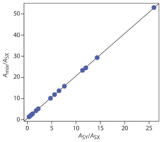
First we need to calculate values for A_mix/A_SX and for A_SY/A_SX. Let’s define X as Co²⁺ and Y as Cr³⁺. For example, at a wavelength of 375 nm A_mix/A_SX is 0.53/0.01, or 53 and A_SY/A_SX is 0.26/0.01, or 26. Completing the calculation for all wavelengths and graphing A_mix/A_SX versus A_SY/A_SX gives the calibration curve shown in Figure \(\PageIndex{2}\). Fitting a straight-line to the data gives a regression model of

\[\frac{A_{\operatorname{mix}}}{A_{S X}}=0.636+2.01 \times \frac{A_{S Y}}{A_{S X}} \nonumber \]

Using the y-intercept, the concentration of Co²⁺ is

\[\frac{C_{X}}{C_{S X}}=\frac{\left[\mathrm{Co}^{2+}\right]}{0.0750 \mathrm{M}}=0.636 \nonumber \]

or [Co²⁺] = 0.048 M; using the slope the concentration of Cr³⁺ is

\[\frac{C_{Y}}{C_{S Y}}=\frac{\left[\mathrm{Cr}^{3+}\right]}{0.0250 \mathrm{M}}=2.01 \nonumber \]

or [Cr³⁺] = 0.050 M.

Figure \(\PageIndex{2}\). Multiwavelength linear regression analysis for the data in Example 14.4.3 .

Exercise 14.4.3

A mixture of \(\text{MnO}_4^{-}\) and \(\text{Cr}_2\text{O}_7^{2-}\), and standards of 0.10 mM KMnO₄ and of 0.10 mM K₂Cr₂O₇ give the results shown in the following table. Determine the composition of the mixture. The data for this problem is from Blanco, M. C.; Iturriaga, H.; Maspoch, S.; Tarin, P. J. Chem. Educ. 1989, 66, 178–180.

\(\lambda\) (nm)	AMn	ACr	Amix
266	0.042	0.410	0.766
288	0.082	0.283	0.571
320	0.168	0.158	0.422
350	0.125	0.318	0.672
360	0.036	0.181	0.366

Answer

Letting X represent \(\text{MnO}_4^{-}\) and letting Y represent \(\text{Cr}_2\text{O}_7^{2-}\), we plot the equation

\[\frac{A_{\operatorname{mix}}}{A_{SX}}=\frac{C_{X}}{C_{SX}}+\frac{C_{Y}}{C_{S Y}} \times \frac{A_{S Y}}{A_{SX}} \nonumber \]

placing A_mix/A_SX on the y-axis and A_SY/A_SX on the x-axis. For example, at a wavelength of 266 nm the value A_mix/A_SX of is 0.766/0.042, or 18.2, and the value of A_SY/A_SX is 0.410/0.042, or 9.76. Completing the calculations for all wavelengths and plotting the data gives the result shown here

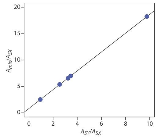
Fitting a straight-line to the data gives a regression model of

\[\frac{A_{\text { mix }}}{A_{\text { SX }}}=0.8147+1.7839 \times \frac{A_{SY}}{A_{SX}} \nonumber \]

Using the y-intercept, the concentration of \(\text{MnO}_4^{-}\) is

\[\frac{C_{X}}{C_{S X}}=0.8147=\frac{\left[\mathrm{MnO}_{4}^{-}\right]}{1.0 \times 10^{-4} \ \mathrm{M} \ \mathrm{MnO}_{4}^{-}} \nonumber \]

or \(8.15 \times 10^{-5}\) M \(\text{MnO}_4^{-}\), and using the slope, the concentration of \(\text{Cr}_2\text{O}_7^{2-}\) is

\[\frac{C_{Y}}{C_{S Y}}=1.7839=\frac{\left[\mathrm{Cr}_{2} \mathrm{O}_{7}^{2-}\right]}{1.00 \times 10^{-4} \ \mathrm{M} \ \text{Cr}_{2} \mathrm{O}_{7}^{2-}} \nonumber \]

or \(1.78 \times 10^{-4}\) M \(\text{Cr}_2\text{O}_7^{2-}\).

Derivative Spectroscopy

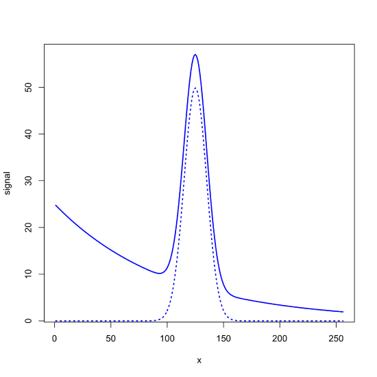
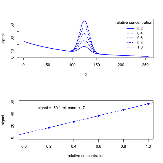
Sometimes our signal is superimposed on a background signal, which complicates our analysis because the measure absorbance has contributions from both our analyte and from the background. For example, the following figure shows a Gaussian signal with a maximum value of 50 centered at \(x = 125\) that is superimposed on an exponential background. The dotted line is the Gaussian signal, which has a maximum value of 50 at \(x = 125\), and the solid line is the signal as measured, which has a maximum value of 57 at \(x = 125\).

Figure \(\PageIndex{3}\): A Gaussian signal (dotted line) superimposed on an exponential background, which gives rise to the measured signal (solid line).

If the background signal is consistent across all samples, then we can analyze the data without first removing its contribution. For example, the following figure shows a set of calibration standards and their resulting calibration curve, for which the y-intercept of 7 gives the offset introduced by the background.

Figure \(\PageIndex{4}\): When the background is the same for all calibration standards and samples, then we can construct a calibration curve without taking into account the presence of the background.

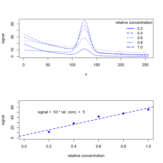
But background signals often are not consistent across samples, particularly when the source of the background is a property of the samples we collect (natural water samples, for example, may have variations in color due to differences in the concentration of dissolved organic matter) or a property of the instrument we are using (such as a variation in source intensity over time). When true, our data may look more like what we see in the following figure, which leads to a calibration curve with a greater uncertainty.

Figure \(\PageIndex{5}\): When the background is not the same for all calibration standards, the quality of the calibration curves suffers, making it less useful for the analysis of samples.

Because the background changes gradually with the values for x while the analyte's signal changes quickly, we can use a derivative to the distinguish between the two. One approach is to calculate and plot the derivative, \(\frac{\Delta y}{\Delta x}\), as a function of \(x\), as shown in Figure \(\PageIndex{6}\). The calibration signal in this case is the difference between the maximum signal and the minimum signal, which are shown by the dotted red lines in the top part of the figure. The fit of the calibration curve to the data and the calibration curve's y-intercept of zero shows that we have successfully compensated for the background signals.

Figure \(\PageIndex{6}\): Taking the derivative of the data in Figure \(\PageIndex{5}\) removes the background signal.