14.2: Absorbing Species
- Page ID
- 365737

\( \newcommand{\vecs}[1]{\overset { \scriptstyle \rightharpoonup} {\mathbf{#1}} } \)
\( \newcommand{\vecd}[1]{\overset{-\!-\!\rightharpoonup}{\vphantom{a}\smash {#1}}} \)
\( \newcommand{\id}{\mathrm{id}}\) \( \newcommand{\Span}{\mathrm{span}}\)
( \newcommand{\kernel}{\mathrm{null}\,}\) \( \newcommand{\range}{\mathrm{range}\,}\)
\( \newcommand{\RealPart}{\mathrm{Re}}\) \( \newcommand{\ImaginaryPart}{\mathrm{Im}}\)
\( \newcommand{\Argument}{\mathrm{Arg}}\) \( \newcommand{\norm}[1]{\| #1 \|}\)
\( \newcommand{\inner}[2]{\langle #1, #2 \rangle}\)
\( \newcommand{\Span}{\mathrm{span}}\)
\( \newcommand{\id}{\mathrm{id}}\)
\( \newcommand{\Span}{\mathrm{span}}\)
\( \newcommand{\kernel}{\mathrm{null}\,}\)
\( \newcommand{\range}{\mathrm{range}\,}\)
\( \newcommand{\RealPart}{\mathrm{Re}}\)
\( \newcommand{\ImaginaryPart}{\mathrm{Im}}\)
\( \newcommand{\Argument}{\mathrm{Arg}}\)
\( \newcommand{\norm}[1]{\| #1 \|}\)
\( \newcommand{\inner}[2]{\langle #1, #2 \rangle}\)
\( \newcommand{\Span}{\mathrm{span}}\) \( \newcommand{\AA}{\unicode[.8,0]{x212B}}\)
\( \newcommand{\vectorA}[1]{\vec{#1}} % arrow\)
\( \newcommand{\vectorAt}[1]{\vec{\text{#1}}} % arrow\)
\( \newcommand{\vectorB}[1]{\overset { \scriptstyle \rightharpoonup} {\mathbf{#1}} } \)
\( \newcommand{\vectorC}[1]{\textbf{#1}} \)
\( \newcommand{\vectorD}[1]{\overrightarrow{#1}} \)
\( \newcommand{\vectorDt}[1]{\overrightarrow{\text{#1}}} \)
\( \newcommand{\vectE}[1]{\overset{-\!-\!\rightharpoonup}{\vphantom{a}\smash{\mathbf {#1}}}} \)
\( \newcommand{\vecs}[1]{\overset { \scriptstyle \rightharpoonup} {\mathbf{#1}} } \)
\( \newcommand{\vecd}[1]{\overset{-\!-\!\rightharpoonup}{\vphantom{a}\smash {#1}}} \)
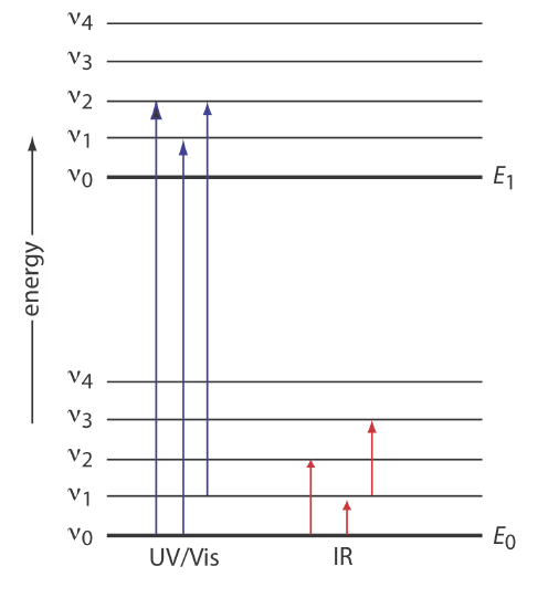
\(\newcommand{\avec}{\mathbf a}\) \(\newcommand{\bvec}{\mathbf b}\) \(\newcommand{\cvec}{\mathbf c}\) \(\newcommand{\dvec}{\mathbf d}\) \(\newcommand{\dtil}{\widetilde{\mathbf d}}\) \(\newcommand{\evec}{\mathbf e}\) \(\newcommand{\fvec}{\mathbf f}\) \(\newcommand{\nvec}{\mathbf n}\) \(\newcommand{\pvec}{\mathbf p}\) \(\newcommand{\qvec}{\mathbf q}\) \(\newcommand{\svec}{\mathbf s}\) \(\newcommand{\tvec}{\mathbf t}\) \(\newcommand{\uvec}{\mathbf u}\) \(\newcommand{\vvec}{\mathbf v}\) \(\newcommand{\wvec}{\mathbf w}\) \(\newcommand{\xvec}{\mathbf x}\) \(\newcommand{\yvec}{\mathbf y}\) \(\newcommand{\zvec}{\mathbf z}\) \(\newcommand{\rvec}{\mathbf r}\) \(\newcommand{\mvec}{\mathbf m}\) \(\newcommand{\zerovec}{\mathbf 0}\) \(\newcommand{\onevec}{\mathbf 1}\) \(\newcommand{\real}{\mathbb R}\) \(\newcommand{\twovec}[2]{\left[\begin{array}{r}#1 \\ #2 \end{array}\right]}\) \(\newcommand{\ctwovec}[2]{\left[\begin{array}{c}#1 \\ #2 \end{array}\right]}\) \(\newcommand{\threevec}[3]{\left[\begin{array}{r}#1 \\ #2 \\ #3 \end{array}\right]}\) \(\newcommand{\cthreevec}[3]{\left[\begin{array}{c}#1 \\ #2 \\ #3 \end{array}\right]}\) \(\newcommand{\fourvec}[4]{\left[\begin{array}{r}#1 \\ #2 \\ #3 \\ #4 \end{array}\right]}\) \(\newcommand{\cfourvec}[4]{\left[\begin{array}{c}#1 \\ #2 \\ #3 \\ #4 \end{array}\right]}\) \(\newcommand{\fivevec}[5]{\left[\begin{array}{r}#1 \\ #2 \\ #3 \\ #4 \\ #5 \\ \end{array}\right]}\) \(\newcommand{\cfivevec}[5]{\left[\begin{array}{c}#1 \\ #2 \\ #3 \\ #4 \\ #5 \\ \end{array}\right]}\) \(\newcommand{\mattwo}[4]{\left[\begin{array}{rr}#1 \amp #2 \\ #3 \amp #4 \\ \end{array}\right]}\) \(\newcommand{\laspan}[1]{\text{Span}\{#1\}}\) \(\newcommand{\bcal}{\cal B}\) \(\newcommand{\ccal}{\cal C}\) \(\newcommand{\scal}{\cal S}\) \(\newcommand{\wcal}{\cal W}\) \(\newcommand{\ecal}{\cal E}\) \(\newcommand{\coords}[2]{\left\{#1\right\}_{#2}}\) \(\newcommand{\gray}[1]{\color{gray}{#1}}\) \(\newcommand{\lgray}[1]{\color{lightgray}{#1}}\) \(\newcommand{\rank}{\operatorname{rank}}\) \(\newcommand{\row}{\text{Row}}\) \(\newcommand{\col}{\text{Col}}\) \(\renewcommand{\row}{\text{Row}}\) \(\newcommand{\nul}{\text{Nul}}\) \(\newcommand{\var}{\text{Var}}\) \(\newcommand{\corr}{\text{corr}}\) \(\newcommand{\len}[1]{\left|#1\right|}\) \(\newcommand{\bbar}{\overline{\bvec}}\) \(\newcommand{\bhat}{\widehat{\bvec}}\) \(\newcommand{\bperp}{\bvec^\perp}\) \(\newcommand{\xhat}{\widehat{\xvec}}\) \(\newcommand{\vhat}{\widehat{\vvec}}\) \(\newcommand{\uhat}{\widehat{\uvec}}\) \(\newcommand{\what}{\widehat{\wvec}}\) \(\newcommand{\Sighat}{\widehat{\Sigma}}\) \(\newcommand{\lt}{<}\) \(\newcommand{\gt}{>}\) \(\newcommand{\amp}{&}\) \(\definecolor{fillinmathshade}{gray}{0.9}\)There are two general requirements for an analyte’s absorption of electromagnetic radiation. First, there must be a mechanism by which the radiation’s electric field or magnetic field can interact with the analyte. For ultraviolet and visible radiation, absorption of a photon changes the energy of the analyte’s valence electrons. The second requirement is that the photon’s energy, \(h \nu\), must exactly equal the difference in energy, \(\Delta E\), between two of the analyte’s quantized energy states. We can use the energy level diagram in Figure \(\PageIndex{1}\) to explain an absorbance spectrum. The lines labeled E0 and E1 represent the analyte’s ground (lowest) electronic state and its first electronic excited state. Superimposed on each electronic energy level is a series of lines representing vibrational energy levels.
UV/Vis Spectra for Molecules and Ions
The valence electrons in organic molecules and polyatomic ions, such as \(\text{CO}_3^{2-}\), occupy quantized sigma bonding (\(\sigma\)), pi bonding (\(\pi\)), and non-bonding (n) molecular orbitals (MOs). Unoccupied sigma antibonding (\(\sigma^*\)) and pi antibonding (\(\pi^*\)) molecular orbitals are slightly higher in energy. Because the difference in energy between the highest-energy occupied molecular orbitals (HOMO) and the lowest-energy unoccupied molecular orbitals (LUMO) corresponds to ultraviolet and visible radiation, absorption of a photon is possible.
Four types of transitions between quantized energy levels account for most molecular UV/Vis spectra. Table \(\PageIndex{1}\) lists the approximate wavelength ranges for these transitions, as well as a partial list of bonds, functional groups, or molecules responsible for these transitions. Of these transitions, the most important are \(n \rightarrow \pi^*\) and \(\pi \rightarrow \pi^*\) because they involve important functional groups that are characteristic of many analytes and because the wavelengths are easily accessible. The bonds and functional groups that give rise to the absorption of ultraviolet and visible radiation are called chromophores.
| transition | wavelength range | examples |
|---|---|---|
| \(\sigma \rightarrow \sigma^*\) | <200 nm | C—C, C—H |
| \(n \rightarrow \sigma^*\) | 160–260 nm | H2O, CH3OH, CH3Cl |
| \(\pi \rightarrow \pi^*\) | 200–500 nm | C=C, C=O, C=N, C≡C |
| \(n \rightarrow \pi^*\) | 250–600 nm | C=O, C=N, N=N, N=O |
Many transition metal ions, such as Cu2+ and Co2+, form colorful solutions because the metal ion absorbs visible light. The transitions that give rise to this absorption are valence electrons in the metal ion’s d-orbitals, which are shown in Figure \(\PageIndex{2}\). For a free metal ion, the five d-orbitals are of equal energy.
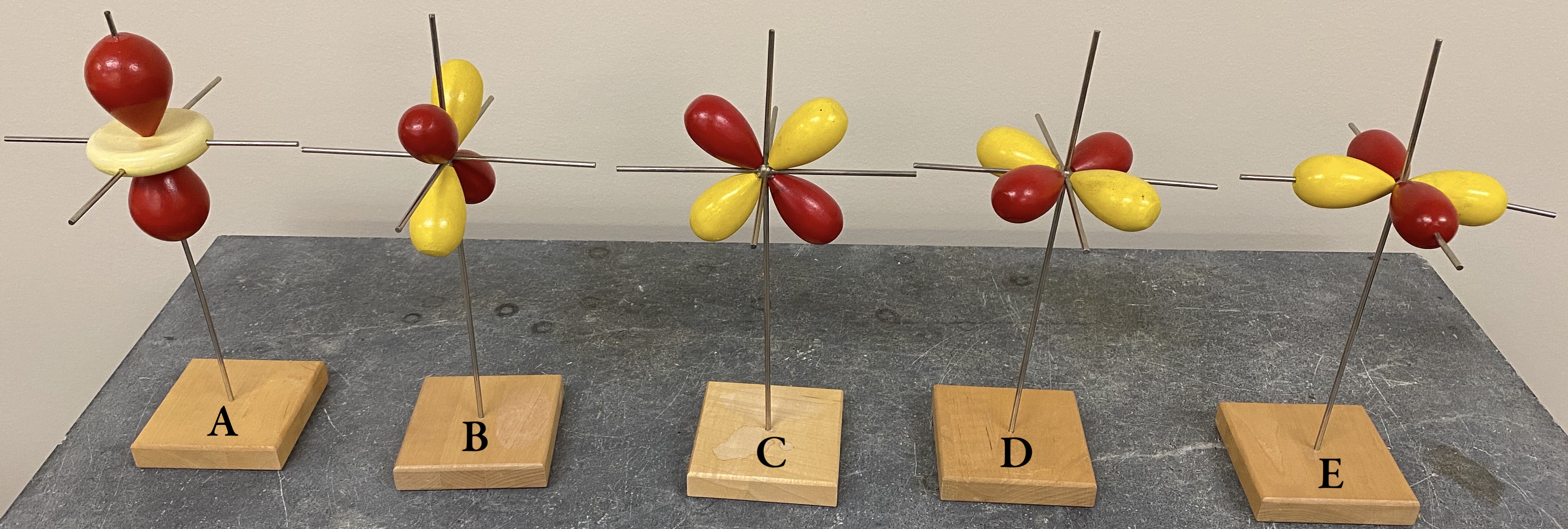
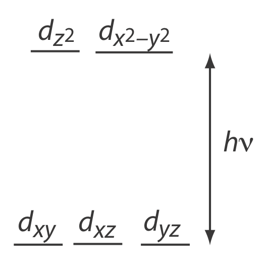
In the presence of a complexing ligand or solvent molecule, however, the d-orbitals split into two or more groups that differ in energy. For example, in an octahedral complex of \(\text{Cu(H}_2\text{O)}_6^{2+}\) the six water molecules, which are aligned with the metal rods in Figure \(\PageIndex{2}\), perturb the d-orbitals into the two groups shown in Figure \(\PageIndex{3}\). The magnitude of the splitting of the \(d\)-orbitals is called the octahedral field strength, \(\Delta_\text{oct}\).
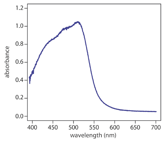
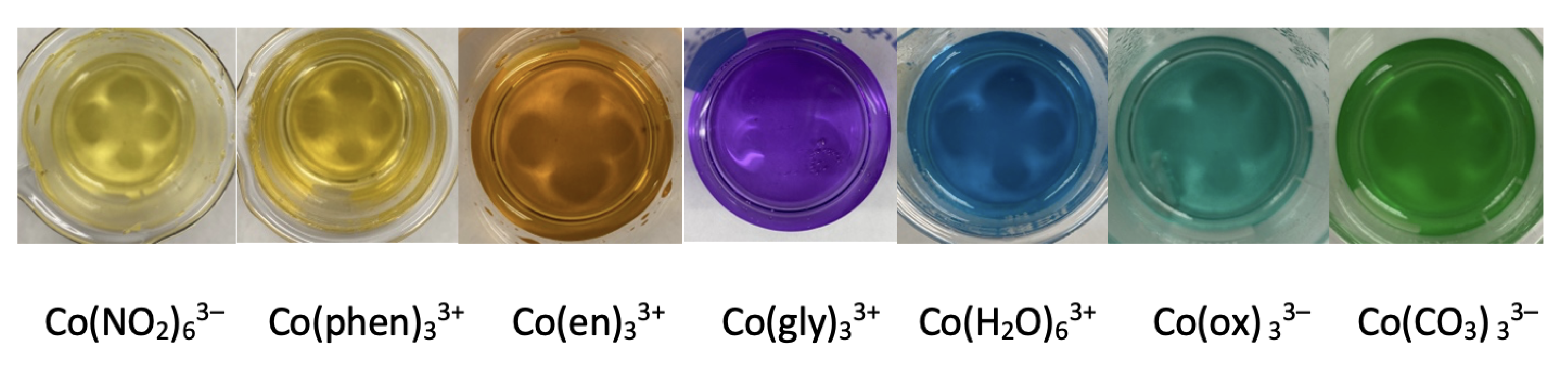
Although the magnitude of the resulting \(d \rightarrow d\) transitions for transition metal ions are relatively weak, solutions of the metal-ligand complexes show distinct colors that depend on the metal ion and the ligand, which affect the magnitude of \(\Delta_\text{oct}\). Figure \(\PageIndex{4}\) shows the variation in color for a series of seven octahedral complexes of Co3+. The spectra for three of these complexes are shown in Figure \(\PageIndex{5}\), which we can use to estimate the relative size of \(\Delta_\text{oct}\). Each of the spectra shows two absorption bands, one near 400 nm and one a somewhat longer wavelength: a shoulder at about 470 nm for phenanthroline, a peak at about 550 nm for glycine, and a peak at about 620 nm for oxalate. Because \(\Delta_\text{oct}\) is inversely proportional to wavelength, the relative magnitude of \(\Delta_\text{oct}\) increases from Co(phen)33+ to Co(glycine)33+ to Co(oxalate)33–. In Figure \(\PageIndex{4}\), the octahedral field strengths of the ligands decrease from Co(NO2)63– to Co(CO3)33–.

A more important source of UV/Vis absorption for inorganic metal–ligand complexes is charge transfer, in which absorption of a photon produces an excited state in which there is transfer of an electron from the metal, M, to the ligand, L.
\[M-L+h \nu \rightarrow\left(M^{+}-L^{-}\right)^{*} \nonumber \]
Charge-transfer absorption is important because it produces very large absorbances. One important example of a charge-transfer complex is that of o-phenanthroline with Fe2+, the UV/Vis spectrum for which is shown in Figure \(\PageIndex{7}\). Charge-transfer absorption in which an electron moves from the ligand to the metal also is possible.