13.4: Instrumentation

Last updated
Save as PDF

Page ID: 365729

\( \newcommand{\vecs}[1]{\overset { \scriptstyle \rightharpoonup} {\mathbf{#1}} } \) \( \newcommand{\vecd}[1]{\overset{-\!-\!\rightharpoonup}{\vphantom{a}\smash {#1}}} \)\(\newcommand{\id}{\mathrm{id}}\) \( \newcommand{\Span}{\mathrm{span}}\) \( \newcommand{\kernel}{\mathrm{null}\,}\) \( \newcommand{\range}{\mathrm{range}\,}\) \( \newcommand{\RealPart}{\mathrm{Re}}\) \( \newcommand{\ImaginaryPart}{\mathrm{Im}}\) \( \newcommand{\Argument}{\mathrm{Arg}}\) \( \newcommand{\norm}[1]{\| #1 \|}\) \( \newcommand{\inner}[2]{\langle #1, #2 \rangle}\) \( \newcommand{\Span}{\mathrm{span}}\) \(\newcommand{\id}{\mathrm{id}}\) \( \newcommand{\Span}{\mathrm{span}}\) \( \newcommand{\kernel}{\mathrm{null}\,}\) \( \newcommand{\range}{\mathrm{range}\,}\) \( \newcommand{\RealPart}{\mathrm{Re}}\) \( \newcommand{\ImaginaryPart}{\mathrm{Im}}\) \( \newcommand{\Argument}{\mathrm{Arg}}\) \( \newcommand{\norm}[1]{\| #1 \|}\) \( \newcommand{\inner}[2]{\langle #1, #2 \rangle}\) \( \newcommand{\Span}{\mathrm{span}}\)\(\newcommand{\AA}{\unicode[.8,0]{x212B}}\)

Basic Components

As covered in Chapter 7, the basic instrumentation for absorbance measurements consists of a source of radiation, a means for selecting the wavelengths to use, a means for detecting the amount of light absorbed by the sample, and a means for processing and displaying the data. In this section we consider two other essential components of an instrument for measuring the absorbance of UV/Vis radiation by molecules: the optical path that connects the source to the detector and a means for placing the sample in this optical path.

Instrument Designs for Molecular UV/Vis Absorption

Frequently an analyst must select from among several different optical paths, the one that is best suited for a particular analysis. In this section we examine several different instruments for molecular absorption spectroscopy with an emphasis on their advantages and limitations.

Filter Photometer

The simplest instrument for molecular UV/Vis absorption is a filter photometer (Figure \(\PageIndex{1}\)), which uses an absorption or interference filter to isolate a band of radiation. The filter is placed between the source and the sample to prevent the sample from decomposing when exposed to higher energy radiation. A filter photometer has a single optical path between the source and detector, and is called a single-beam instrument. The instrument is calibrated to 0% T while using a shutter to block the source radiation from the detector. After opening the shutter, the instrument is calibrated to 100% T using an appropriate blank. The blank is then replaced with the sample and its transmittance measured. Because the source’s incident power and the sensitivity of the detector vary with wavelength, the photometer is recalibrated whenever the filter is changed. Photometers have the advantage of being relatively inexpensive, rugged, and easy to maintain. Another advantage of a photometer is its portability, making it easy to take into the field. Disadvantages of a photometer include the inability to record an absorption spectrum and the source’s relatively large effective bandwidth, which limits the calibration curve’s linearity.

The percent transmittance varies between 0% and 100%. We use a blank to determine P₀, which corresponds to 100%T. Even in the absence of light the detector records a signal. Closing the shutter allows us to assign 0%T to this signal. Together, setting 0% T and 100%T calibrates the instrument. The amount of light that passes through a sample produces a signal that is greater than or equal to 0%T and smaller than or equal to 100%T.

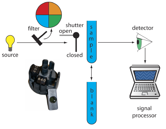
Schematic diagram of a filter photometer.

Figure \(\PageIndex{1}\). Schematic diagram of a filter photometer. The analyst either inserts a removable filter or the filters are placed in a carousel, an example of which is shown in the photographic inset. The analyst selects a filter by rotating it into place.

Single-Beam Spectrophotometer

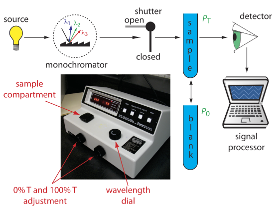
An instrument that uses a monochromator for wavelength selection is called a spectrophotometer. The simplest spectrophotometer is a single-beam instrument equipped with a fixed-wavelength monochromator (Figure \(\PageIndex{2}\)). Single-beam spectrophotometers are calibrated and used in the same manner as a photometer. One example of a single-beam spectrophotometer is Thermo Scientific’s Spectronic 20D+, which is shown in the photographic insert to Figure \(\PageIndex{2}\). The Spectronic 20D+ has a wavelength range of 340–625 nm (950 nm when using a red-sensitive detector), and a fixed effective bandwidth of 20 nm. Battery-operated, hand-held single-beam spectrophotometers are available, which are easy to transport into the field. Other single-beam spectrophotometers also are available with effective bandwidths of 2–8 nm. Fixed wavelength single-beam spectrophotometers are not practical for recording spectra because manually adjusting the wavelength and recalibrating the spectrophotometer is awkward and time-consuming. The accuracy of a single-beam spectrophotometer is limited by the stability of its source and detector over time.

Double-Beam Spectrophotometer

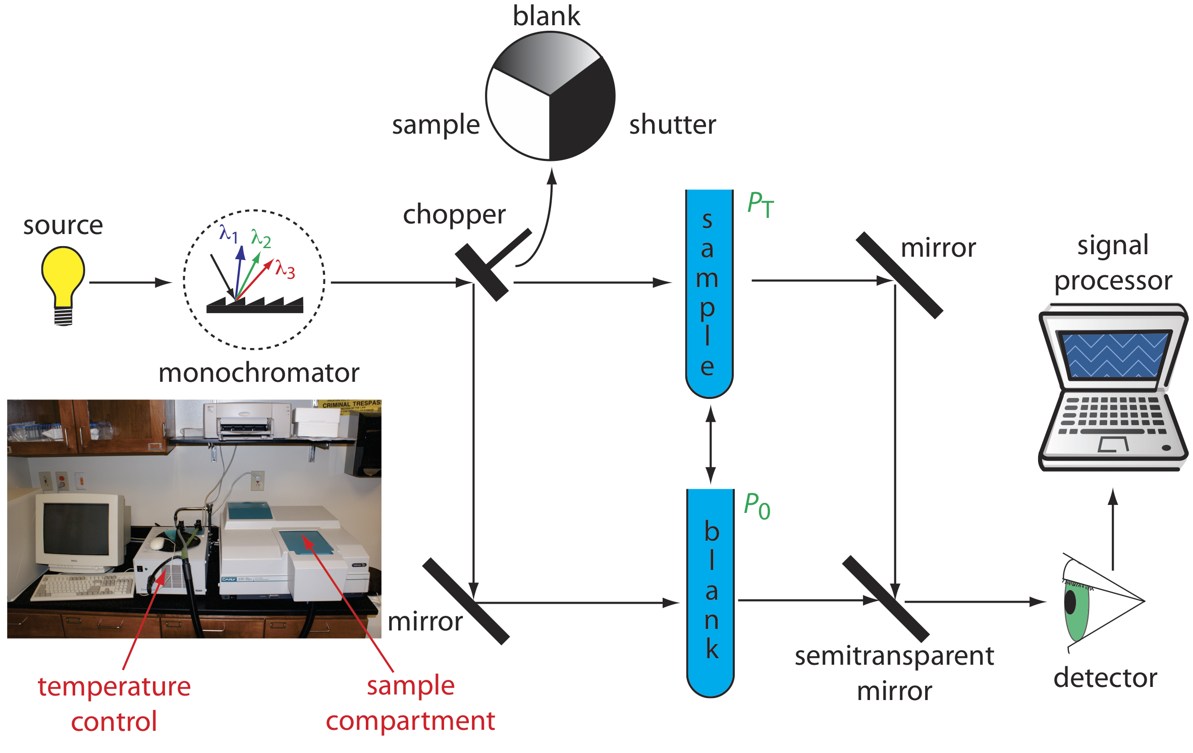
The limitations of a fixed-wavelength, single-beam spectrophotometer is minimized by using a double-beam spectrophotometer (Figure \(\PageIndex{3}\)). A chopper controls the radiation’s path, alternating it between the sample, the blank, and a shutter. The signal processor uses the chopper’s speed of rotation to resolve the signal that reaches the detector into the transmission of the blank, P₀, and the sample, P_T. By including an opaque surface as a shutter, it also is possible to continuously adjust 0%T. The effective bandwidth of a double-beam spectrophotometer is controlled by adjusting the monochromator’s entrance and exit slits. Effective bandwidths of 0.2–3.0 nm are common. A scanning monochromator allows for the automated recording of spectra. Double-beam instruments are more versatile than single-beam instruments, being useful for both quantitative and qualitative analyses, but also are more expensive and not particularly portable.

Diode Array Spectrometer

An instrument with a single detector can monitor only one wavelength at a time. If we replace a single photomultiplier with an array of photodiodes, we can use the resulting detector to record a full spectrum in as little as 0.1 s. In a diode array spectrometer the source radiation passes through the sample and is dispersed by a grating (Figure \(\PageIndex{4}\)). The photodiode array detector is situated at the grating’s focal plane, with each diode recording the radiant power over a narrow range of wavelengths. Because we replace a full monochromator with just a grating, a diode array spectrometer is small and compact.

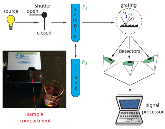
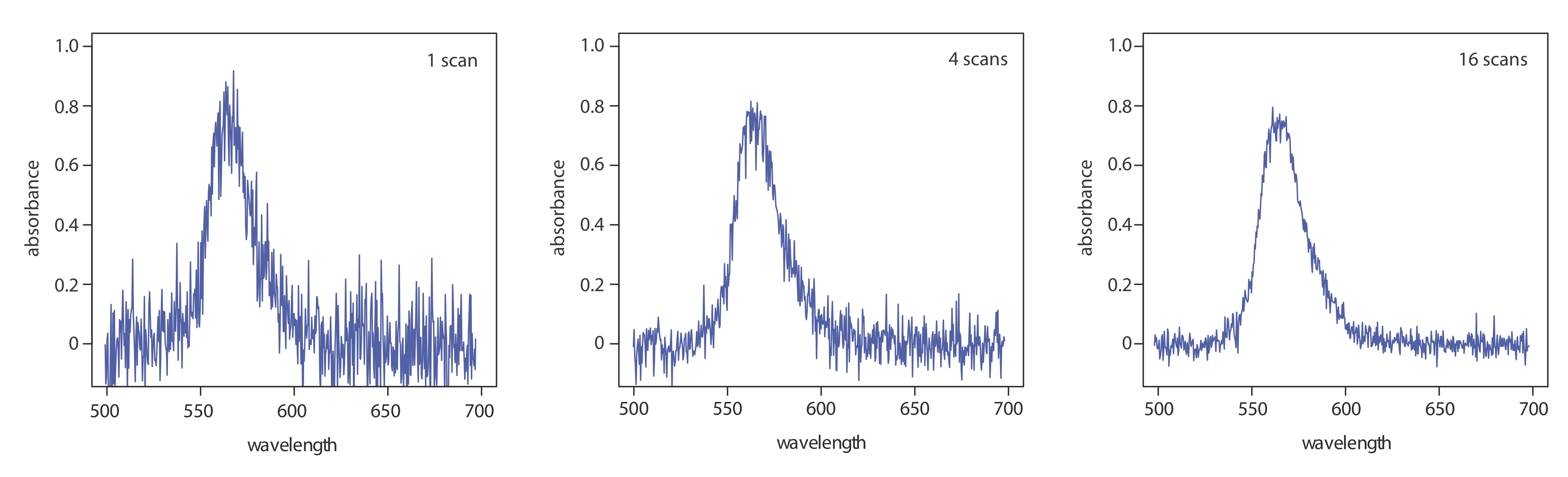
Figure \(\PageIndex{4}\). Schematic diagram of a diode array spectrophotometer. The photographic insert shows a typical instrument. Note that the 50-mL beaker provides a sense of scale. Because the spectrometer is small and compact, it is easy to transport into the field.

One advantage of a diode array spectrometer is the speed of data acquisition, which allows us to collect multiple spectra for a single sample. Individual spectra are added and averaged to obtain the final spectrum. This signal averaging improves a spectrum’s signal-to-noise ratio. If we add together n spectra, the sum of the signal at any point, x, increases as nS_x, where S_x is the signal. The noise at any point, N_x, is a random event, which increases as \(\sqrt{n} N_x\) when we add together n spectra. The signal-to-noise ratio after n scans, (S/N)_n is

\[\left(\frac{S}{N}\right)_{n}=\frac{n S_{x}}{\sqrt{n} N_{x}}=\sqrt{n} \frac{S_{x}}{N_{x}} \nonumber \]

where S_x/N_x is the signal-to-noise ratio for a single scan. The impact of signal averaging is shown in Figure \(\PageIndex{5}\). The first spectrum shows the signal after one scan, which consists of a single, noisy peak. Signal averaging using 4 scans and 16 scans decreases the noise and improves the signal-to-noise ratio. One disadvantage of a photodiode array is that the effective bandwidth per diode is roughly an order of magnitude larger than that for a high quality monochromator.

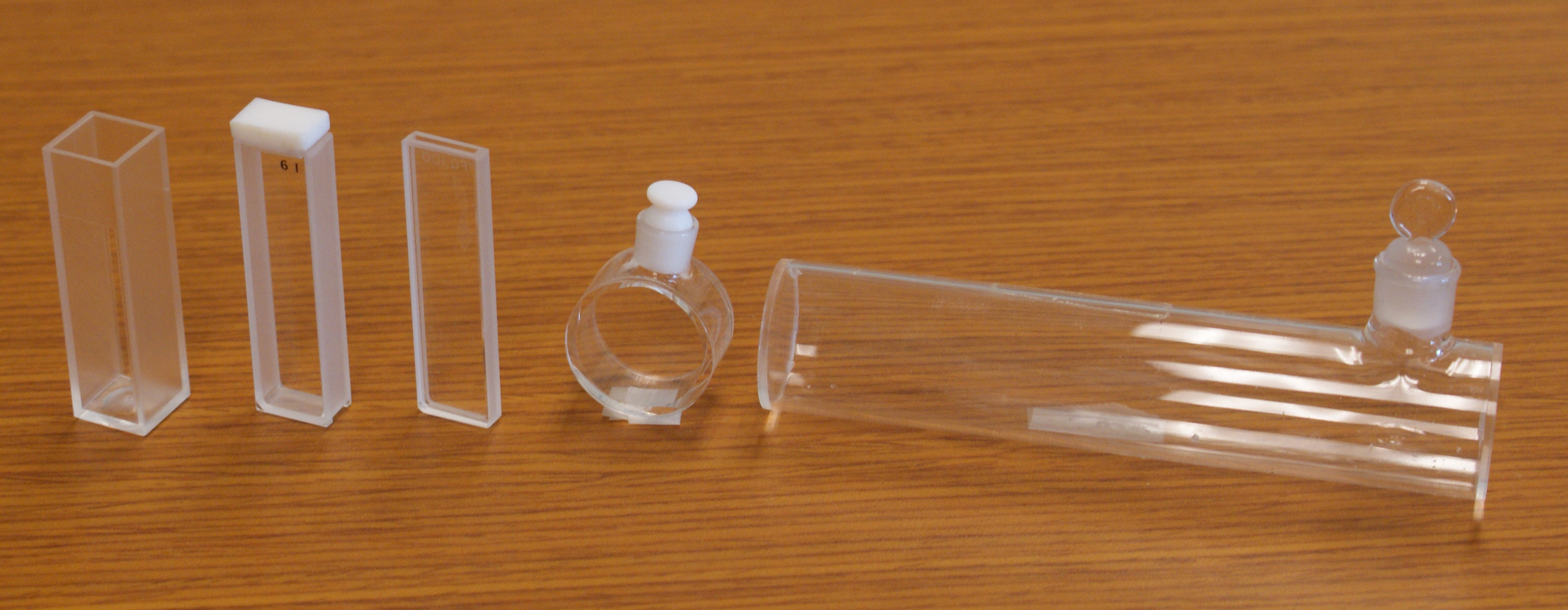
Figure \(\PageIndex{5}\). Effect of signal averaging on a spectrum’s signal-to-noise ratio. From top to bottom: spectrum for a single scan; average spectrum after four scans; and average spectrum after adding 16 scans.

Sample Cells

The sample compartment provides a light-tight environment that limits stray radiation. Samples normally are in a liquid or solution state, and are placed in cells constructed with UV/Vis transparent materials, such as quartz, glass, and plastic (Figure \(\PageIndex{6}\)). A quartz or fused-silica cell is required when working at a wavelength <300 nm where other materials show a significant absorption. The most common pathlength is 1 cm (10 mm), although cells with shorter (as little as 0.1 cm) and longer pathlengths (up to 10 cm) are available. Longer pathlength cells are useful when analyzing a very dilute solution or for gas samples. The highest quality cells allow the radiation to strike a flat surface at a 90^o angle, minimizing the loss of radiation to reflection. A test tube often is used as a sample cell with simple, single-beam instruments, although differences in the cell’s pathlength and optical properties add an additional source of error to the analysis.

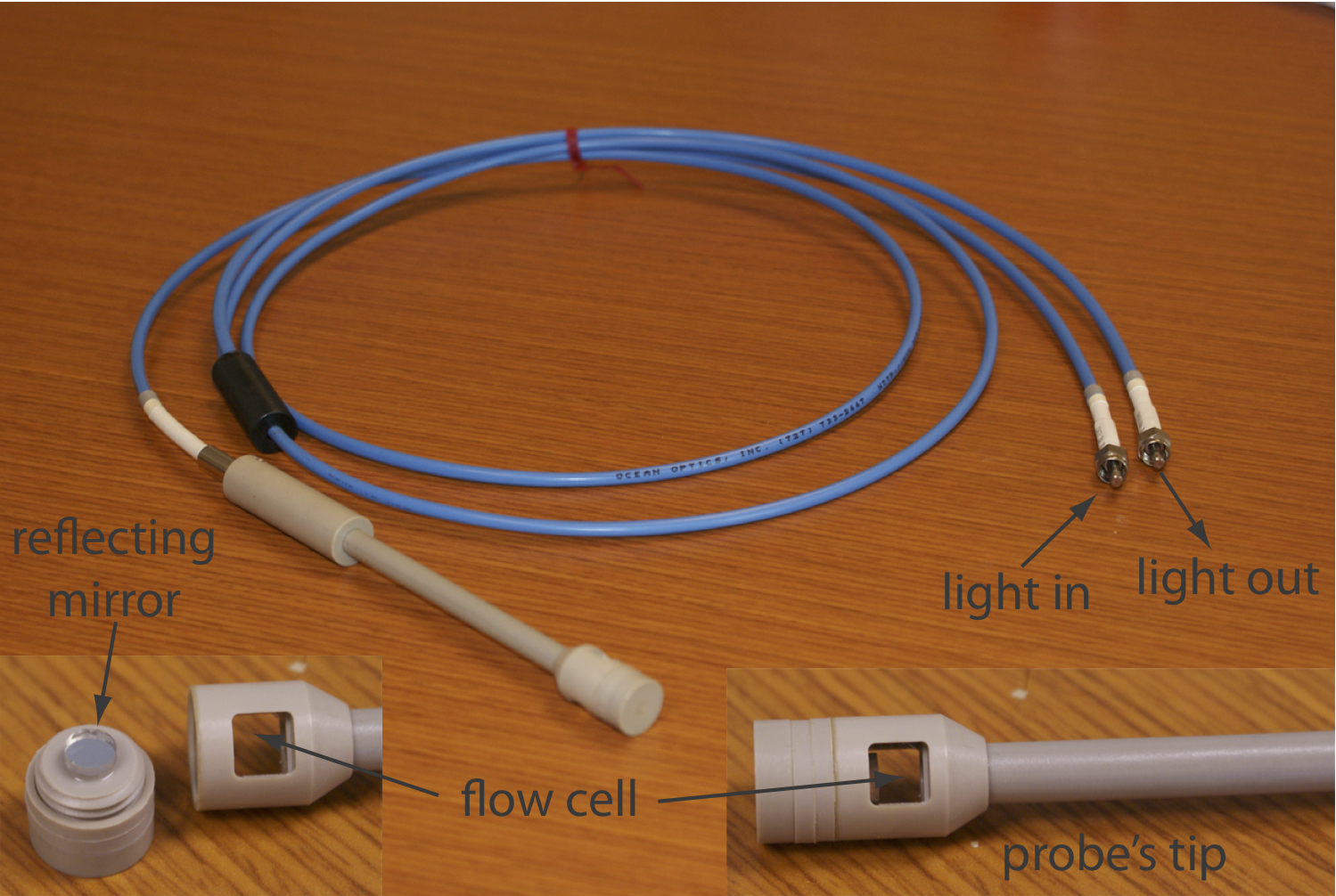
If we need to monitor an analyte’s concentration over time, it may not be possible to remove samples for analysis. This often is the case, for example, when monitoring an industrial production line or waste line, when monitoring a patient’s blood, or when monitoring an environmental system, such as stream. With a fiber-optic probe we can analyze samples in situ. An example of a remote sensing fiber-optic probe is shown in FFigure \(\PageIndex{7}\). The probe consists of two bundles of fiber-optic cable. One bundle transmits radiation from the source to the probe’s tip, which is designed to allow the sample to flow through the sample cell. Radiation from the source passes through the solution and is reflected back by a mirror. The second bundle of fiber-optic cable transmits the nonabsorbed radiation to the wavelength selector. Another design replaces the flow cell shown in Figure \(\PageIndex{7}\) with a membrane that contains a reagent that reacts with the analyte. When the analyte diffuses into the membrane it reacts with the reagent, producing a product that absorbs UV or visible radiation. The nonabsorbed radiation from the source is reflected or scattered back to the detector. Fiber optic probes that show chemical selectivity are called optrodes [(a) Seitz, W. R. Anal. Chem. 1984, 56, 16A–34A; (b) Angel, S. M. Spectroscopy 1987, 2(2), 38–48].

Figure \(\PageIndex{7}\). Example of a fiber-optic probe. The inset photographs at the bottom of the figure provide close-up views of the probe’s flow cell and the reflecting mirror.