13.3: Effect of Noise on Transmittance and Absorbance Measurements

In absorption spectroscopy, precision is limited by indeterminate errors—primarily instrumental noise—which are introduced when we measure absorbance. Precision generally is worse for low absorbances where P₀ ≈ P_T, and for high absorbances where P_T approaches 0. We might expect, therefore, that precision will vary with transmittance.

We can derive an expression between precision and transmittance by rewriting Beer's law as

\[C=-\frac{1}{\varepsilon b} \log T \label{noise1} \]

and completing a propagation of uncertainty (see the Appendicies for a discussion of propagation of error), which gives

\[s_{c}=-\frac{0.4343}{\varepsilon b} \times \frac{s_{T}}{T} \label{noise2} \]

where s_T is the absolute uncertainty in the transmittance. Dividing Equation \ref{noise2} by Equation \ref{noise1} gives the relative uncertainty in concentration, s_C/C, as

\[\frac{s_c}{C}=\frac{0.4343 s_{T}}{T \log T} \nonumber \]

If we know the transmittance’s absolute uncertainty, then we can determine the relative uncertainty in concentration for any measured transmittance.

Determining the relative uncertainty in concentration is complicated because s_T is a function of the transmittance. As shown in Table \(\PageIndex{1}\), three categories of indeterminate instrumental error are observed [Rothman, L. D.; Crouch, S. R.; Ingle, J. D. Jr. Anal. Chem. 1975, 47, 1226–1233].

Table \(\PageIndex{1}\). Effect of Indeterminate Errors on Relative Uncertainty in Concentration

category	sources of indeterminate error	relative uncertainty in concentration
\(s_T = k_1\)	%T readout resolution noise in thermal detectors	\(\frac{s_{C}}{C}=\frac{0.4343 k_{1}}{T \log T}\)
\(s_T = k_2 \sqrt{T^2 + T}\)	noise in photon detectors	\(\frac{s_{C}}{C}=\frac{0.4343 k_{2}}{\log T} \sqrt{1+\frac{1}{T}}\)
\(s_T = k_3 T\)	positioning of sample cell fluctuations in source intensity	\(\frac{s_{C}}{C}=\frac{0.4343 k_{3}}{\log T}\)

A constant s_T is observed for the uncertainty associated with reading %T on a meter’s analog or digital scale, both common on less-expensive spectrophotometers. Typical values are ±0.2–0.3% (a k₁ of ±0.002–0.003) for an analog scale and ±0.001% a (k₁ of ±0.00001) for a digital scale. A constant s_T also is observed for the thermal transducers used in infrared spectrophotometers. The effect of a constant s_T on the relative uncertainty in concentration is shown by curve A in Figure \(\PageIndex{1}\). Note that the relative uncertainty is very large for both high absorbances and low absorbances, reaching a minimum when the absorbance is 0.4343. This source of indeterminate error is important for infrared spectrophotometers and for inexpensive UV/Vis spectrophotometers. To obtain a relative uncertainty in concentration of ±1–2%, the absorbance is kept within the range 0.1–1.

Figure \(\PageIndex{1}\). Percent relative uncertainty in concentration as a function of absorbance for the categories of indeterminate errors in Table \(\PageIndex{10.3}\). A: k₁ = ±0.0030; B: k₂ = ±0.0030; and C: k₃= ±0.0130. The dashed lines correspond to the minimum uncertainty for curve A (absorbance of 0.4343) and for curve B (absorbance of 0.963).

Values of s_T are a complex function of transmittance when indeterminate errors are dominated by the noise associated with photon detectors. Curve B in Figure \(\PageIndex{1}\) shows that the relative uncertainty in concentration is very large for low absorbances, but is smaller at higher absorbances. Although the relative uncertainty reaches a minimum when the absorbance is 0.963, there is little change in the relative uncertainty for absorbances between 0.5 and 2. This source of indeterminate error generally limits the precision of high quality UV/Vis spectrophotometers for mid-to-high absorbances.

Finally, the value of s_T is directly proportional to transmittance for indeterminate errors that result from fluctuations in the source’s intensity and from uncertainty in positioning the sample within the spectrometer. The latter is particularly important because the optical properties of a sample cell are not uniform. As a result, repositioning the sample cell may lead to a change in the intensity of transmitted radiation. As shown by curve C in Figure \(\PageIndex{1}\), the effect is important only at low absorbances. This source of indeterminate errors usually is the limiting factor for high quality UV/Vis spectrophotometers when the absorbance is relatively small.

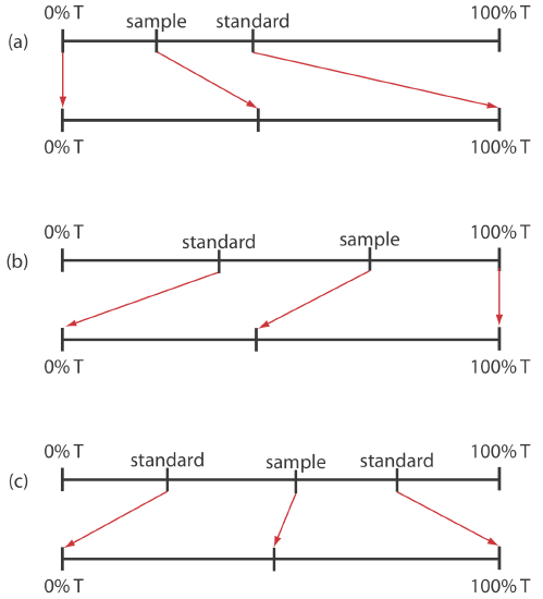
When the relative uncertainty in concentration is limited by the %T readout resolution, it is possible to improve the precision of the analysis by redefining 100% T and 0% T. Normally 100% T is established using a blank and 0% T is established while preventing the source’s radiation from reaching the detector. If the absorbance is too high, precision is improved by resetting 100% T using a standard solution of analyte whose concentration is less than that of the sample (Figure \(\PageIndex{2}a\)). For a sample whose absorbance is too low, precision is improved by redefining 0% T using a standard solution of the analyte whose concentration is greater than that of the analyte (Figure \(\PageIndex{2}b\)). In this case a calibration curve is required because a linear relationship between absorbance and concentration no longer exists. Precision is further increased by combining these two methods (Figure \(\PageIndex{2}c\)). Again, a calibration curve is necessary since the relationship between absorbance and concentration is no longer linear.

Figure 13.3.17 . Methods for improving the precision of absorption methods: (a) high-absorbance method; (b) low-absorbance method; (c) maximum precision method.