12.2: Instrument Components

Atomic X-ray spectrometry has the same needs as other forms of optical spectroscopy: a source of X-rays, a means for isolating a desired range of wavelengths of X-rays, a means for detecting the X-rays, and a means for converting the signal at the transducer into a meaningful number.

X-Ray Sources

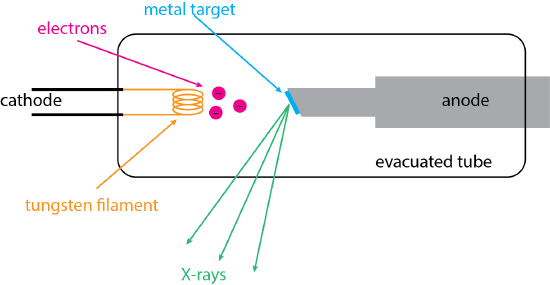
The most important source of X-rays is the X-ray tube, a basic diagram of which is shown in Figure \(\PageIndex{1}\). A beam of electrons (shown in red) from a heated tungsten filament (shown in orange) serves as a cathode with a negative potential. The electrons are drawn toward an anode that has a positive potential. The tip of the anode is made from a metal target (shown in blue) that will produce X-rays (shown in green) with the desired wavelengths when struck by the electron beam. Typical metal targets include tungsten, molybdenum, silver, copper, iron, and cobalt. The filament and the target metal are housed inside an evacuated tube. The emitted X-rays exit the tube through an optical window.

Figure \(\PageIndex{1}\): Schematic diagram showing the key parts of an X-ray tube. See text for details.

Any material that is naturally radioactive emits characteristic X-rays that potentially can serve as a source of X-rays that another species can absorb. For example, in the absorption spectrum for molybdenum (see Figure 18.1.4) the \(\text{K}_{\alpha}\) line has a wavelength of 0.62 Å, which corresponds to an energy of 20.0 kV. A radioactive source with an emission line that has a wavelength slightly longer than 0.62 Å (between, for example, 0.5 Å and 0.6 Å) is sufficient. One possibility is ¹⁰⁹Cd, which emits X-rays with a wavelength of 0.56 Å, or an energy of 22 kV.

X-Ray Filters and Monochromators

A filter and a monochromator are designed to take a broad range of emission from a source and narrow the range of wavelengths that reach the sample. Figure \(\PageIndex{2}\) shows how to accomplish this using an absorption filter. The blue line shows the emission spectrum for a sample that includes two lines—the \(\text{K}_{\alpha}\) line and the \(\text{K}_{\beta}\) line—superimposed on a broad continuum. The green line shows the absorption spectrum for a different element whose K edge falls in between the sample's \(\text{K}_{\alpha}\) and \(\text{K}_{\beta}\) lines. In this case the K edge filter removes most of the continuum and the \(\text{K}_{\beta}\) line, allowing just the \(\text{K}_{\alpha}\) line and a small amount of the continuum to reach the sample.

Figure \(\PageIndex{2}\): Illustration of how an X-ray filter works by comparing the absorbance spectrum for the filter (in green) to the emission spectrum of the source (in blue). See the text for additional details.

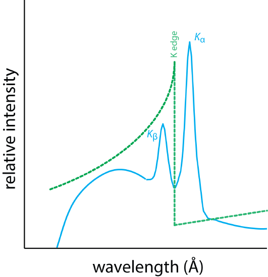
Figure \(\PageIndex{3}\) shows the basic design for an X-ray monochromator, which can operate in either an absorption mode, in which X-rays from the source pass through the sample before entering the monochromator, or in an emission mode, in which X-rays from the source excite the sample and fluorescent emission is sampled at 90°.

Figure \(\PageIndex{3}\): Illustration of an X-ray monochromator. The black circle shows the location of the sample and the X-ray source, which can take one of two configurations and experiments: absorption mode or emission mode. See text for additional details.

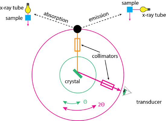
In either mode, the X-rays pass through a collimator that focuses them onto a crystal where the X-rays undergo diffraction. X-rays are collected by a second collimator before arriving at the transducer. To scan the source, the crystal rotates through an angle of \(\theta\); the transducer must rotate twice as fast, traversing an angle of \(2 \theta\) to maintain an identical angle between the source and the transducer.

An X-ray monochromator's effective range is determined by the properties of the crystal used for diffraction. We know from Chapter 12.1 that

\[n \lambda = 2 d \sin \theta \label{diffract1} \]

where \(n\) is the diffraction order, \(\lambda\) is the wavelength, \(\theta\) is the X-ray's angle of incidence, and \(d\) is the spacing between the crystal's layers. The practical limit for the angle depends on the monochromator's design, but typically \(\theta\) is 7.5° to 75° (or \(2 \theta\) angles of 15° to 150°). A common crystal is LiF, which has a spacing of 2.01 Å; thus, it provides a wavelength range from a lower limit of

\[ \lambda = 2 d \sin \theta = 2 \times 2.01 \text{ Å} \times \sin(7.5^{\circ}) = 0.52 \text{ Å} \nonumber \]

to an upper limit of

\[ \lambda = 2 d \sin \theta = 2 \times 2.01 \text{ Å} \times \sin(75^{\circ}) = 3.9 \text{ Å} \nonumber \]

when \(n = 1\). This range of wavelengths is sufficient to study the elements K to Cd using their \(\text{K}_{\alpha}\) lines.

X-Ray Transducers

The most common transducers for atomic X-ray spectrometry are the flow proportional counter, the scintillation counter, and the Si(Li) semiconductor. All three transducers act as photon counters.

Photon Counting

The most common transducer for measuring atomic absorbance and atomic emission of ultraviolet and visible light is a photomultiplier tube. As we learned in Chapter 7, a photon strikes a photosensitive surface and generates several electrons. These electrons collide with a series of dynodes, each collision of which generates additional electrons. This amplification of one photon into 10⁶–10⁷ electrons results in a steady-state current that we can measure. When the intensity of radiation from the source is smaller, as it is with X-rays, then it is possible to store the electrons in a capacitor that, when discharged, provides a pulsed signal that carries information about the photons.

Flow Proportional Counters

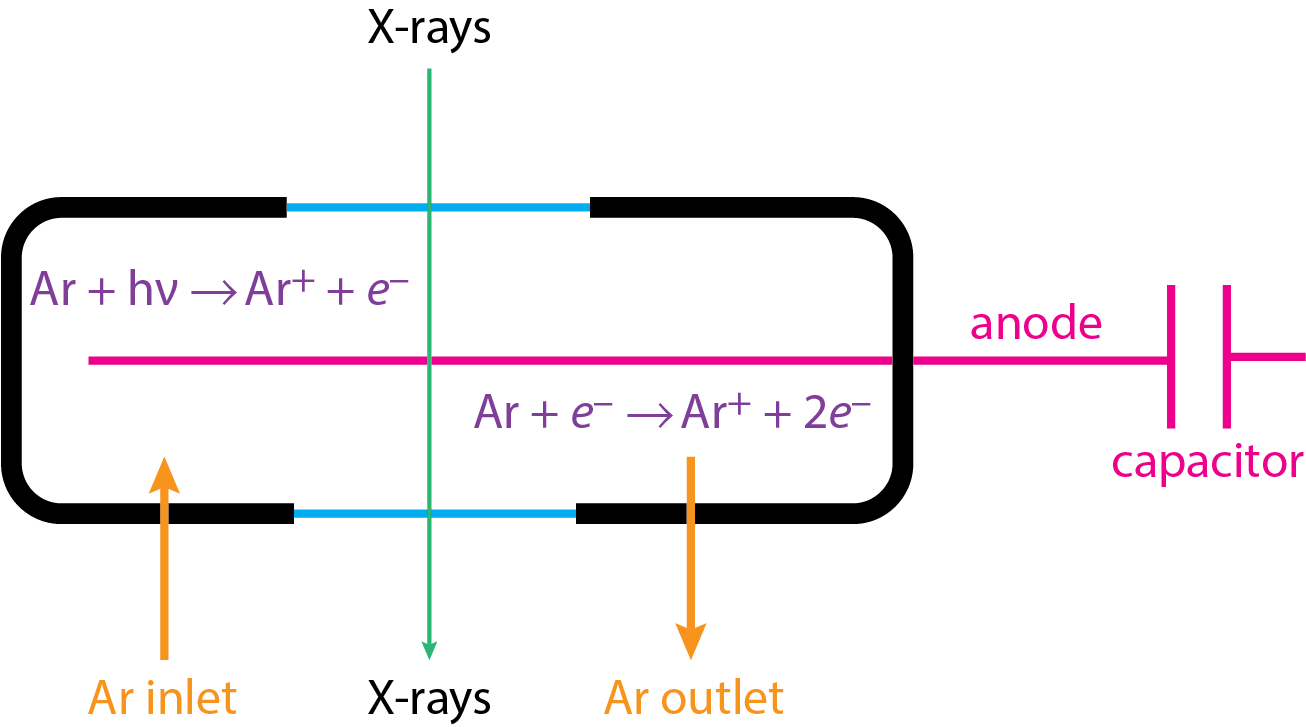
Figure \(\PageIndex{4}\) shows the basic structure of a flow proportional counter. The transducer's cell has an inlet and an outlet for creating the flow of argon gas. The cell has windows made from an X-ray transparent materials, such as beryllium. X-rays enter the cell and, as shown by the reaction in the upper left, ionizes the argon, generating a photoelectron. This photoelectron is sufficiently energetic that it further ionizes the argon, as shown by the reaction in the lower right. The result is an amplification of a single photon into as many as 10,000 electrons. These electrons are drawn to a tungsten wire that is held at a positive charge, and then flow into a capacitor. Discharging the capacitor gives a pulsed signal whose height is proportional to the initial number of electrons and, therefore, to the energy, frequency, and wavelength of the photons.

Figure \(\PageIndex{4}\): Schematic diagram of a flow proportional cell for photon counting. See text for details.

Scintillation Counters

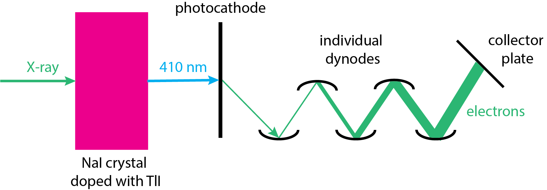
A flow proportional counter is not an efficient transducer for shorter wavelength (lower energy) X-rays that are likely to pass through the cell without being absorbed by the argon gas, leading to a reduction in the signal. In this case we can use a scintillation counter. Figure \(\PageIndex{5}\) shows how this works. X-ray photons are focused onto a single crystal of NaI that is doped with a small amount, approximately 0.2%, of Tl⁺ as an iodide salt. Absorption of the X-rays results in the fluorescent emission of multiple photons of visible light with a wavelength of 410 nm. Each of these photons falls on the photocathode of a photomultiplier, eventually producing a voltage pulse. Each pulse corresponds to a single photon with an energy that is proportional to the pulse's height.

Figure \(\PageIndex{5}\): Schematic diagram of a scintillation counter. See text for details.

Semiconductor Transducers

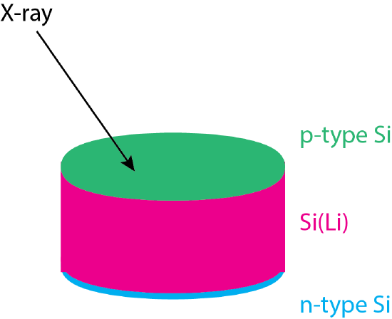
In Chapter 7.5 we introduced the use of the pn junction of a silicon semiconductor as a transducer for optical spectroscopy. Absorption of a photon of sufficient energy results in the formation of an electron-hole pair. Movement of the electron through the n-layer and movement of the hole through the p-region generates a current that is proportional to the number of photons reaching the detector. Figure \(\PageIndex{6}\) shows the structure of the semiconductor used in monitoring X-rays, which consists of a p-type layer and an n-type layer on either side of single crystal of silicon doped with lithium or germanium. The Si(Li) layer has the same role here as Ar has in the flow proportional counter. An X-ray photon that enters into the Si(Li) layer generates electron-hole pairs leading to a measurable current that is proportional to the energy of the X-ray.

Figure \(\PageIndex{6}\): Structure of a Si(Li) semiconductor transducer.

X-Ray Signal Processors

The flow proportional counter, scintillation counter, and semiconductor transducers pass a stream of pulses to the signal processor where pulse-height selector is used to isolate only those pulses of interest and a pulse-height analyzer is used to summarize the distribution of pulses.

Pulse-Height Selectors

Not all pulses measured by the transducer are of interest. For example, pulses with small heights are likely to be noise and pulses with large heights may be a higher-order (\(n > 1\)) diffraction of shorter, and more energetic wavelengths. Figure \(\PageIndex{7}\) shows the basic details of how pulse-height selector works. The pulse-height selector is set to pass only those pulse heights that are between a lower limit and an upper limit. The figure shows three pulses, one that is too small (in blue), one that is too large (in red), and one that we wish to keep (in green). The pulses run through two channels, one that removes only the blue signal and one that retains only the red signal. The latter signal is inverted and combined with the signal from the other channel. Because the red signal has a different sign in the two channels, it, too, is removed, leaving only the one pulse height that meets the criteria for selection.

Figure \(\PageIndex{7}\): Illustration of how a pulse-height selector works. Three pulses arrive at the signal processor shown in blue, green, and red with heights greater than the baseline (shown as 0). The pulse-height selector is set to remove all pulses that have a height less than that shown by the low pass limit, and to remove all pulses that have a height greater than the high pass limit. In this case, the low pass filter removes the pulse in blue, and the high pass filter removes all but the pulse in green. The latter is then inverted and then added to the former giving a final signal that contains the one pulse that falls within the two limits.

Having removed pulses with heights that are too small or too large, the remaining pulses are analyzed by counting the number of pulses that share a range of pulse heights. Each unique range of pulse heights is called a channel and corresponds to a specific energy of the photons. A spectrum is a plot showing the count of pulses as function of the energy of the photons.