12.1: Fundamental Principles

In Chapter 6 we introduced the electromagnetic spectrum and the characteristic properties of photons, such as the wavelengths, the frequencies, and the energies of ultraviolet, visible, and infrared light. The wavelength range for photons of X-ray radiation extends from approximately 0.01 nm to 10 nm. Although we are used to reporting a photon's wavelength in nanometers, for historical reasons the wavelength of an X-ray photon usually is reported in angstroms (for which the symbol is Å) where 1 Å = 0.1 nm; thus the wavelength range of 0.01 nm to 10 nm for X-ray radiation also is expressed as 0.1 Å to 100 Å. This range of wavelengths corresponds to a range of frequencies from approximately \(3 \times 10^{19} \text{ s}^{-1}\) to \(3 \times 10^{16} \text{ s}^{-1}\), and a range of energies from \(2 \times 10^{-19} \text{ J}\) to \(2 \times 10^{-17} \text{ J}\).

Sources of X-Rays

There are three routine ways to generate X-rays, each of which is covered in this section: we can bombard a suitable metal with a beam of high-energy electrons, we can use one X-ray to stimulate the emission of additional X-rays through fluorescence, and we can use a radioactive isotope that emits X-rays as it decays.

Obtaining X-Rays From Electron Beam Sources

An electron beam is created by heating a tungsten wire filament to a temperature at which it releases electrons. These electrons are pulled toward a metal target by applying an accelerating voltage between the metal target and the tungsten wire. The result is the broad continuum of X-ray emission in Figure \(\PageIndex{1}\). The source of this continuous emission spectrum is the reduction in the kinetic energy of the electrons as they collide with the metal target. The loss of kinetic energy results in the production of photons over a broad range of wavelengths and is known as Bremsstrahlung, or braking radiation.

Note

In earlier chapters we divided the sources of photons into two broad groups: continuous sources, such as a tungsten lamp, that produce photons at all wavelengths between a lower limit and an upper limit, and line sources, such as a hollow cathode lamp, that produce photons for one or more discrete wavelengths. The sources used to generate X-rays also generate continuum and/or line spectra.

Figure \(\PageIndex{1}\): X-ray emission from a metal target using an electron beam. The voltage listed above each curve is the accelerating voltage used to create the electron beam. Each accelerating voltage has a minimum wavelength, \(\lambda_0\), below which emission does not occur. The dashed line shows \(\lambda_0\) for an accelerating voltage of 40 kV.

The lower wavelength limit for X-ray emission, identified here as \(\lambda_0\), is the maximum possible loss of kinetic energy, KE, and is equal to

\[KE = \frac{hc}{\lambda_0} = Ve \label{lmin} \]

where h is Planck's constant, c is the speed of light, V is the accelerating voltage, and e is the charge on the electron. The product of the accelerating voltage and the charge on the electron is the kinetic energy of the electrons. Solving Equation \ref{lmin} for \(\lambda_0\) gives

\[\lambda_0 = \frac{hc}{Ve} = \frac{12.398 \text{ kV Å}}{V} \label{lambdamin2} \]

where \(\lambda_0\) is in angstroms and V is in kilovolts. Note that Equation \ref{lmin} and Equation \ref{lambdamin2} do not include any terms that depend on the target metal, which means that for any accelerating voltage, \(\lambda_0\) is the same for all metal targets. Table \(\PageIndex{1}\) gives values of \(\lambda_0\) that span the range of accelerating voltages in Figure \(\PageIndex{1}\).

Table \(\PageIndex{1}\). Shortest wavelength of continuous X-ray emission when using an electron beam as a function of its accelerating voltage.

accelerating voltage (kV)	\(\lambda_0\) (Å)
20	0.62
25	0.50
30	0.41
35	0.35
40	0.31
45	0.28
50	0.25

If we apply a sufficiently large accelerating voltage, then the emission spectrum will consist of both a continuum spectrum and a line spectrum, as we see in Figure \(\PageIndex{2}\) with molybdenum as the target metal. The spectrum consists of both a continuum similar to that in Figure \(\PageIndex{1}\), and two lines, one at a wavelength of 0.63 Å and one at a wavelength of 0.71 Å. The source of these lines is the emission of X-rays from excited state ions that form when a sufficiently high-energy electron from the electron beam removes an electron from an atomic orbital close to the nucleus. As electrons in atomic orbitals at a greater distance from the nucleus drop into the atomic orbital with a vacancy, they release their extra energy as a photon.

Although the background emission from the continuum is the same for all metal targets, the energy for the lines have values that are characteristic for different metals because the energy to remove an electron varies from element-to-element, increasing with atomic number. For example, an accelerating voltage of at least

\[V = \frac{12.398 \text{ kV Å}}{0.61 Å} = 20 \text{ kV} \nonumber \]

is needed to generate the line spectrum for molybdenum in Figure \(\PageIndex{2}\).

Figure \(\PageIndex{2}\): The X-ray emission spectrum for molybdenum using an electron beam with an accelerating voltage of 35 kV. The spectrum consists of both a continuum similar to that in Figure \(\PageIndex{1}\) and two lines, one at a wavelength of 0.63 Å and one at a wavelength of 0.71 Å.

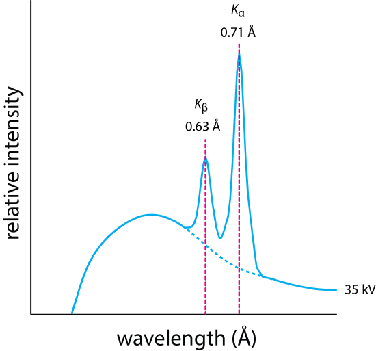
The characteristic emission lines for molybdenum in Figure \(\PageIndex{2}\) are identified as \(K_{\alpha}\) and \(K_{\beta}\), a notation with which you may not be familiar. The simplified energy level diagram in Figure \(\PageIndex{3}\) will help us understand this notation. Each arrow in this energy-level diagram shows a transition in which an electron moves from an orbital at greater distance from the nucleus to an orbital closer to the nucleus. The letters K, L, and M correspond to the principal quantum number n, which has values of 1, 2, 3... that indicate the initial vacancy created by the collision of the ion beam with the target metal. The Greek symbols \(\alpha\), \(\beta\), and \(\gamma\) indicate the source of the electron that fills this vacancy in terms of its change in the principal quantum number, \(\Delta n\). An electron moving from n = 2 to n = 1 and an electron moving from n = 4 to n = 3 have the same designation of \(\alpha\). The emission line in Figure \(\PageIndex{2}\) identified as \(K_{\beta}\), therefore, is the result of an electron in the n = 3 shell moving into a vacancy in the n = 1 shell \(K\).

Figure \(\PageIndex{3}\): Simplified energy-level diagram showing the nomenclature for identifying characteristic X-ray lines.

Note

Why is Figure \(\PageIndex{3}\) a simplified energy-level diagram? For each n > 1 there is more than one atomic orbital. When n = 2 there are three energy levels: one that corresponds to l = 0, one that corresponds to l = 1 and m_l = 0, and one that corresponds to l = 1 and m_l = ±1. The allowed transitions to the n = 1 energy levels requires a change in the value for l; thus, we expect to find two emission lines from n = 2 to n = 1 instead of the one shown in Figure \(\PageIndex{3}\). These two lines, which we can identify as \(\text{K}_{\alpha 1}\) and \(\text{ K}_{\alpha 2}\), generally are sufficiently close in value that they are not resolved in the X-ray emission spectrum. For example, \(\text{K}_{\alpha 1} = 0.709\) and \(\text{ K}_{\alpha 2} = 0.714\) for molybdenum. You can find a table of X-ray emission lines here.

Obtaining X-Rays From Fluorescent Sources

When an atom in an excited state emits a photon as a means of returning to a lower energy state, how we describe the process depends on the source of energy that created the excited state. When excitation is the result of thermal energy, we call the process atomic emission. When excitation is the result of the absorption of a photon, we call the process atomic fluorescence. In X-ray fluorescence, excitation is brought about using photons from a source of continuous X-ray radiation. More details on X-ray fluorescence are provided later in this chapter.

Obtaining X-Rays From Radioactive Sources

Atoms that have the same number of protons but a different number of neutrons are isotopes. To identify an isotope we use the notation \({}_Z^A E\), where E is the element’s atomic symbol, Z is the element’s atomic number, and A is the element’s atomic mass number. Although an element’s different isotopes have the same chemical properties, their nuclear properties are not identical. The most important difference between isotopes is their stability. The nuclear configuration of a stable isotope remains constant with time. Unstable isotopes, however, disintegrate spontaneously, emitting radioactive decay particles as they transform into a more stable form.

An element’s atomic number, Z, is equal to the number of protons and its atomic mass, A, is equal to the sum of the number of protons and neutrons. We represent an isotope of carbon-13 as \(_{6}^{13} \text{C}\) because carbon has six protons and seven neutrons. Sometimes we omit Z from this notation—identifying the element and the atomic number is repetitive because all isotopes of carbon have six protons and any atom that has six protons is an isotope of carbon. Thus, ¹³C and C–13 are alternative notations for this isotope of carbon.

Radioactive particles can decay in several ways, one of which results in the emission of X-rays. For example, ⁵⁵Fe can capture an electron and undergo a process in which a proton becomes a neutron, becoming ⁵⁵Mn and releasing the excess energy as a \(\text{K}_{\alpha}\) X-ray. We will not give further consideration to radioactive sources of atomic X-ray emission; see Chapter 32, however, for a further discussion of radioactive methods of analysis.

X-Ray Absorption

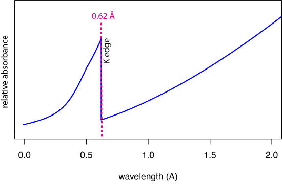
Figure \(\PageIndex{4}\) shows a portion of molybdenum's X-ray absorption spectrum over the same range of wavelengths as shown in Figure \(\PageIndex{2}\) for its emission spectrum. Both spectra are relatively simple: the emission spectrum consists of two lines superimposed on a continuum background, and the absorbance spectrum consists of a single line, identified here as the K edge.

Figure \(\PageIndex{4}\): A portion of the X-ray absorption spectrum for molybdenum.

The Absorption Process

If an X-ray photon is of sufficient energy, then its absorbance by an atom results in the ejection of an electron from one of the atom's innermost atomic orbitals, which you may recognize as the production of a photoelectron. For molybdenum, a wavelength of 0.62 Å (an energy of 20.0 kV) is needed to eject a photoelectron from the K shell (n = 1). At this wavelength the probability of absorption is at is greatest. At shorter wavelengths (greater energies) there is sufficient energy to eject the electron, however, the probability of absorption decreases and the relative absorbance decreases slowly. The abrupt decrease in absorbance for wavelengths larger than 0.62 Å—this abrupt decrease is the source of the term edge—happens because the photons no longer have sufficient energy to eject an electron from the K shell. The slow increasing absorbance at wavelengths greater than the K edge is the result of ejecting electrons from the L shell, which has edges at 4.3 Å, 4.7 Å, and 4.9 Å.

Note

The simplified energy level diagram in \(\PageIndex{3}\) shows only one energy level for n = 2 (the L shell). As we noted earlier, there are three energy levels when n = 2: one that corresponds to l = 0, one that corresponds to l = 1 and m_l = 0, and one that corresponds to l = 1 and m_l = ±1. The three edges corresponding to these energy levels are identified as L_I, L_II, and L_III.

Beer's Law and X-Ray Absorption

When a source of X-rays passes through a sample with a thickness of x, the following equation holds

\[A = -\ln \frac{P}{P_0} = \mu_{\text{M}} \rho x \label{beerxray} \]

where A is the absorbance, \(P_0\) is the power of the X-ray source incident on the sample, \(P\) is the power of the X-ray source after it passes through the sample, \(\mu_{\text{M}}\) is the sample's mass absorption coefficient and \(\rho\) is the sample's density. You may have noticed the similarity between this equation and the equation for Beer's law that we first encountered in Chapter 6

\[A = -\ln \frac{P}{P_0} = \epsilon b C \label{beer} \]

where \(\epsilon\) is the molar absorptivity, \(b\) is the pathlength, and \(C\) is molar concentration. Note that both density (g/mL) and molarity (mol/L) are a measure of concentration that expresses the amount of the absorbing material present in the sample.

X-Ray Fluorescence

When an electron is ejected from a shell near the nucleus by the absorption of an X-ray, the vacancy created is eventually filled when an electron at a greater distance from the nucleus moves down. Because it takes more energy to eject an electron and create a vacancy than is returned by the movement of other electrons into the vacancy, the resulting fluorescent emission of X-rays is always at wavelengths that are longer (lower energy) than the wavelength that was absorbed. We see this in Figure \(\PageIndex{4}\) and Figure \(\PageIndex{1}\) for molybdenum where it absorbs an X-ray with a wavelength of 0.62 Å and emits X-rays with wavelengths of 0.63 Å and 0.71 Å.

X-Ray Diffraction

When an X-ray beam is focused onto a sample that has a regular (crystalline) pattern of atoms in three dimensions, some of the radiation scatters from the surface and some of the radiation passes through to the next layer of atoms where the combination of scattering and passing through continues. As a result of this process, the radiation undergoes diffraction in which X-rays of some wavelengths appear to reflect off the surface while X-rays of other wavelengths do not. The conditions the result in diffraction are easy to understand using the diagram in Figure \(\PageIndex{5}\).

Figure \(\PageIndex{5}\): Illustration showing the diffraction of X-rays from an ordered crystalline sample. See the text for additional details.

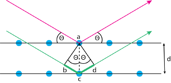
The red and green arrows are two parallel beams of X-rays that are focused on an ordered crystalline solid that consists of a layered repeatable pattern of atoms shown by the blue circles. The two beams of X-rays encounter the solid at an angle of \(\theta\). The X-ray shown in red scatters off of the first layer, exiting at the same angle of \(\theta\). The X-ray shown in green penetrates to the second layer where it undergoes scattering, exiting at the same angle of \(\theta\). We know from the superposition of waves (see Chapter 6) that the two beams of X-rays will remain in phase, and thus experience constructive interference, only if the additional distance traveled by the green wave—the sum of the line segments \(\overline{bc}\) and \(\overline{cd}\)—is an integer multiple of the wavelength; thus

\[\overline{bc} + \overline{cd} = n \lambda \label{bragg1} \]

We also know that the length of the line segments \(\overline{bc}\) and \(\overline{cd}\) are given by

\[\overline{bc}= \overline{cd} = d \sin \theta \label{bragg2} \]

where \(d\) is the distance between the crystal's layers. Combining Equation \ref{bragg1} and Equation \ref{bragg2} gives

\[n \lambda = 2 d \sin \theta \label{bragg3} \]

Rearranging Equation \ref{bragg3} shows that we will observe diffraction only at angles that satisfy the equation

\[\sin \theta = \frac{n \lambda}{2d} \label{bragg4} \]