12.3: Atomic X-Ray Fluorescence Methods

In X-ray fluorescence a source of X-rays—emission from an X-ray tube or emission from a radioactive element—is used to excite the atoms of an analyte in a sample. These excited-state atoms return to their ground state by emitting X-rays, the process we know as fluorescence. The wavelengths of these emission lines are characteristic of the elements that make up the sample; thus, atomic X-ray fluorescence is a useful method for both a qualitative analysis and a quantitative analysis.

Instruments

In the previous section we covered the basic components that make up an atomic X-ray spectrometer: a source of X-rays, a means for isolating those wavelengths of interest, a transducer to measure the intensity of fluorescence, and a signal processor to convert the transducer's signal into a useful measurement. How we string these units together is the subject of this section in which we consider two ways to acquire a sample's spectrum: wavelength dispersive instruments and energy dispersive instruments.

Wavelength Dispersive Instruments

A wavelength dispersive instrument relies on diffraction using a monochromator, such as that in Figure 12.2.3, to select the analytical wavelength. A sequential wavelength dispersive instrument uses a single monochromator. The monochromator's crystal and transducer are set to the desired angles—\(\theta\) for the diffracting crystal and \(2 \theta\) for the transducer—for the analyte of interest and the fluorescence intensity measured for 1-100 s. The monochromator is adjusted for the next analyte and the process repeated until the analysis for all analytes is complete. Analyzing a sample for 20 analytes may take 30 min or more.

A simultaneous, or multichannel, wavelength dispersive instrument contains as many as 30 crystals and transducers, each at a fixed angle that is preset for an analyte of interest. Each individual channel has a dedicated transducer and pulse-height selector and analyzer. Analysis of a complex sample with many analytes requires less than a minute. This is similar to the multichannel ICP used in atomic emission (see Figure 10.1.5).

Energy Dispersive Instruments

An energy dispersive instrument eschews a scanning monochromator and, instead, uses a semiconductor transducer to analyze the fluorescent emission by the determining the energies of the emitted photons. As each photon reaches the transducer as a pulse of electrons, its height is measured and converted into the photon's energy. The result is a spectrum showing a count of photons with the same energy as a function of the energy. The collection of data is very fast: if it takes 25 µs to complete the collection and processing of a single photon, then the instrument can count 40,000 photons each second (40 kcps, or kilo counts per second). One limitation to an energy dispersive instrument is its limited resolution with respect to energy. An instrument that operates with 2048 channels—that is, an instrument that divides the energies into 2048 bins—and that processes photons with energies up to 20 keV, has a resolution of approximately 10 eV per channel. Because it does not rely on a monochromator, an energy dispersive instrument occupies a smaller footprint, and portable, hand-held versions are available.

Qualitative Analysis

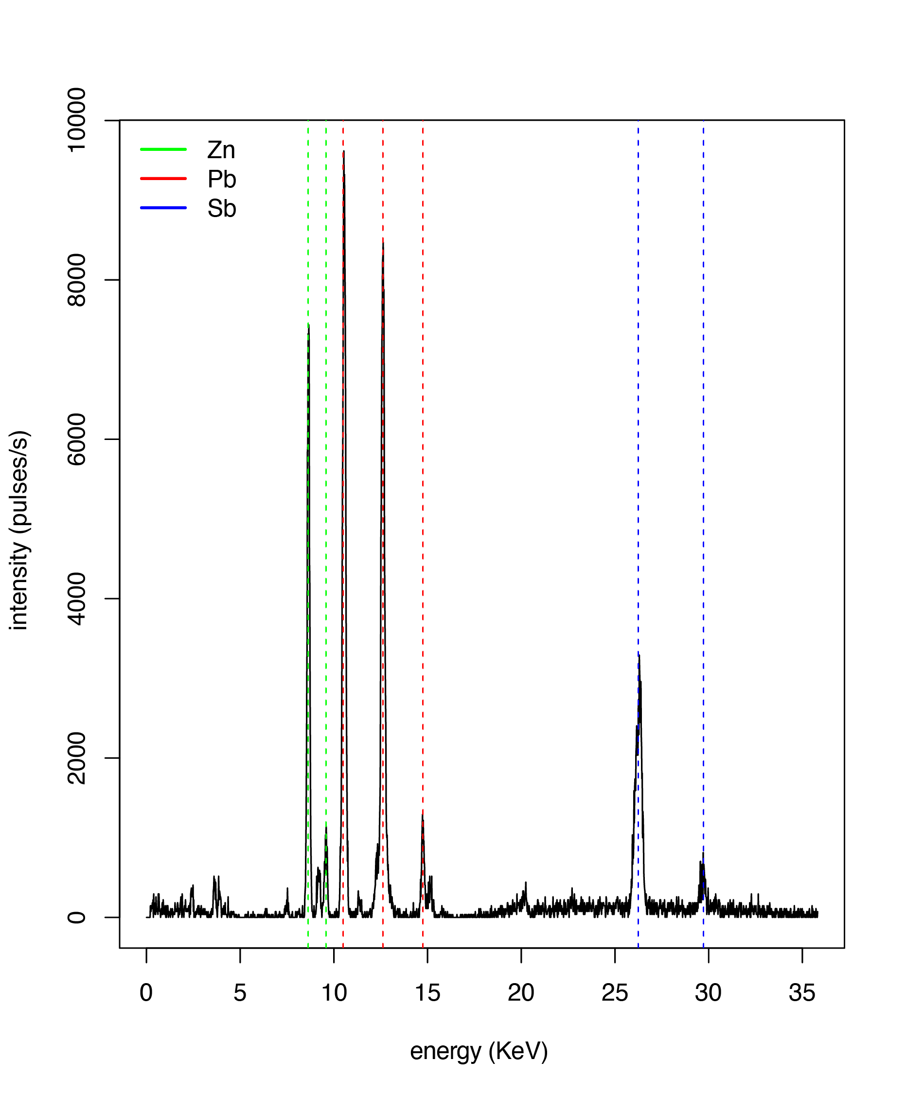
Figure \(\PageIndex{1}\) shows the X-ray fluorescence spectrum for the yellow pigment known as naples yellow, the major elements of which are zinc, lead, and antimony. It is easy to identify the major elements in the sample by matching the energies of the individual lines to the published emission lines of the elements, which are available in many on-line sources. For example, the first line highlighted in this spectrum is at an energy of 8.66 KeV, which is close to the \(\text{K}_{\alpha}\) line for Zn at 8.64 KeV, and the last highlighted line is at an energy of 29.97 KeV, which is close to the \(\text{K}_{\beta}\) line for Sb of 29.7 KeV.

Figure \(\PageIndex{1}\): Energy dispersive XRF of the pigment naples yellow, a lead antimonate that also contains zinc. The spectrometer's energy scale was calibrated using the \(\text{K}_{\alpha}\) line for ²⁶Fe at 6.4 KeV and the \(\text{K}_{\alpha}\) line for ⁴²Mo at 17.44 eV. The emission lines for zinc (\(\text{K}_{\alpha}\) and \(\text{K}_{\beta}\)) are shown in green, the lines for lead (\(\text{L}_{\alpha}\), \(\text{L}_{\beta}\), and \(\text{L}_{\gamma}\)) are shown in red, and the lines for antimony (\(\text{K}_{\alpha}\) and \(\text{K}_{\beta}\)) are shown in blue. The original data is available here.

Quantitative Analysis

A semi-quantitative analysis is possible if we assume that there is a linear relationship between the intensity of an element's emission line and its %w/w concentration in the sample. The intensity of emission from a pure sample or the element, \(I_\text{pure}\), is measured along with the intensity of emission for the element in a sample, \(I_\text{sample}\), and the %w/w calculated as

\[\% \text{w/w} = \frac {I_\text{sample}} {I_\text{pure}} \label{semiquant} \]

Equation \ref{semiquant} is essentially a one-point standardization that makes the significant assumption that the intensity of fluorescent emission is independent of the matrix in which the analyte sits. When this is not true, then errors of \(2 \text{-} 3 \times\) are likely.

Matrix Effects

For fluorescent emission to occur, the analyte must first absorb a photon that can eject a photoelectron. For Equation \ref{semiquant} to hold, the photons that initiate the fluorescent emission must come from the source only. If other elements within the sample's matrix produced fluorescent emission with sufficient energy to eject photoelectrons from the analyte, then the total fluorescence increases and we overestimate the analyte's concentration. If an element in the matrix absorbs the X-rays from the source more strongly than the analyte, then the analyte's total fluorescence becomes smaller and we underestimate the analyte's concentration. There are three common strategies for compensating for matrix effects.

External Standards with Matrix Matching. Instead of using a single, pure sample for the calibration, we prepare a series of standards with different concentrations of the analyte. By matching, as best we can, the matrix of the standards to the matrix of the samples, we can improve the accuracy of a quantitative analysis. This assumes, of course, that we have sufficient knowledge of our sample's matrix.

Internal Standards. An internal standard is an element that we add to the standards and samples so that its concentration is the same in each. If the analyte and the internal standard experience similar matrix effects, then the ratio of their intensities is proportional to the ratio of their concentrations

\[\frac{I_\text{analyte, sample}}{I_\text{int std, sample}} = K \times \frac{C_\text{analyte, sample}}{C_\text{int std, sample}} \label{intstd} \]

Dilution. A third approach is to dilute the samples and standards by adding a quantity of non-absorbing or poorly absorbing material. Dilution has the effect of minimizing the difference in the matrix of the original samples and standards.