6.3: Quantum Mechanical Properties of Electromagnetic Radiation

In the last section, we considered properties of electromagnetic radiation that are consistent with identifying light as a wave. Other properties of light, however, cannot be explained by a model that treats it as a wave; instead, we need to consider a model that treats light as a system of discrete particles, which we call photons.

The Photoelectric Effect

As shown in Figure \(\PageIndex{1}\), in a photoelectric cell, a metal, such as sodium, is held under vacuum and exposed to electromagnetic radiation, which enters the cell through an optical window. If the frequency of the radiation is sufficient, electrons escape from the metal with a kinetic energy that we can measure; we call these photoelectrons. If the photocell's anode is held at a potential that is positive relative to the potential applied to the cathode, the photoelectrons move from the cathode to the anode, generating a current that is measured by an ammeter. If the voltage applied to the anode is made sufficiently negative, the electrons eventually fail to reach the anode and the current decreases to zero. The voltage needed to stop the flow of electrons is called the stopping voltage.

Figure \(\PageIndex{1}\): Illustration of a photoelectric cell. The photocathode is fashioned from or coated with a metal and placed in an evacuated cell along with an anode. Electromagnetic radiation is focused on the photocathode and, if it has sufficient energy, the metal emits electrons with a kinetic energy that depends on the metal and the frequency of the electromagnetic radiation. The potential applied to the photocathode and the anode determine whether the electrons reach the anode; if they do, then a current flows, which is measured by the ammeter.

In a photoelectron spectrum we vary the frequency and intensity of the electromagnetic radiation and observe their effect on either the number of photoelectrons released (measured as a current) or the energy of the photoelectrons released (measured by their kinetic energy). A typical set of experiments are shown in Figure \(\PageIndex{2}a\) using Na and in Figure \(\PageIndex{2}b\) using Na, Zn, and Cu. The data show several interesting features. First, we see in Figure \(\PageIndex{2}a\) that the intensity of the light source has no effect on the minimum frequency of light needed to eject a photoelectron from Na—we call this the threshold frequency—but that a high intensity source of electromagnetic radiation results in the release of a greater number of photoelectrons and, therefore, a greater current than for a lower intensity source. Second, we see in Figure \(\PageIndex{2}b\) that different metals have different threshold frequencies, but that once we exceed each metal's threshold frequency, the change in the kinetic energy of the photoelectrons with increasing frequency yields lines of equal slopes.

Figure \(\PageIndex{2}\): The two types of photoelectric effect experiments. In (a) we measure the current that flows as we change the intensity and the frequency of the electromagnetic radiation. In (b) we measure the kinetic energy of the photoelectrons as a function of the frequency of the electromagnetic radiation.

We can explain these experimental observations if we assume that the source of electromagnetic energy has an energy, \(E_\text{ER}\), that does two things: it overcomes the energy that binds the photoelectron to the metal, \(E_\text{BE}\), and it imparts the remaining energy into the photoelectron's kinetic energy, \(E_\text{KE}\), where ER means electromagnetic radiation, BE means binding energy and KE means kinetic energy.

\[E_\text{KE} = E_\text{ER} - E_\text{BE} \nonumber \]

A wave model for electromagnetic radiation is insufficient to explain the photoelectric effect because when it strikes the metal the radiation's energy would be distributed across all atoms on the surface, none of which would then receive an energy that exceeds the photoelectron's binding energy. Instead, the results in Figure \(\PageIndex{2}\) make sense only if we assume that light consists of discrete particles with energies that are a function of frequency or wavelength

\[E_\text{ER} = h \nu = \frac{hc}{\lambda} \label{qm} \]

where \(h\) is Plank's constant. This leave us with the following equation relating kinetic energy, the energy of the photon, and the binding energy of the electron.

\[E_\text{KE} = h \nu - E_\text{BE} \nonumber \]

Note that the slope of the lines in Figure \(\PageIndex{2}b\) is Plank's constant.

Energy States

Equation \ref{qm} is central to the particle, or quantum mechanical model of the atom in which we understand that chemical species—atoms, ions, molecules—exist only in discrete states, each with a single, well-defined energy. A wave, on the other hand, can take on any energy. A simple image is the possible energies of a ball as it rolls down a ramp (wave) or a staircase (particle), as in Figure \(\PageIndex{3}\).

Figure \(\PageIndex{3}\). The energy of a ball is measured by its height relative to its final position, shown in blue. When a ball rolls down a ramp, as in (a), it can take on any energy between its initial and final energies. When a ball rolls down a staircase, as in (b), it can take only certain discrete energies. The ball in (b) is said to be quantized.

When an atom, ion, or molecule moves between two of these discrete states, the difference in energy, \(\Delta E\), is given by

\[\Delta E = h \nu = \frac{hc}{\lambda} \nonumber \]

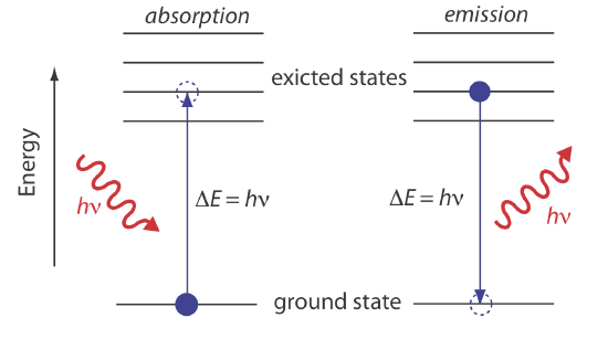
In absorption spectroscopy a photon is absorbed by an atom, ion, or molecule, which undergoes a transition from a lower-energy state to a higher-energy, or excited state (Figure \(\PageIndex{4}a\)). The reverse process, in which an atom, ion, or molecule emits a photon as it moves from a higher-energy state to a lower energy state (\(\PageIndex{4}b\)), is called emission.

Figure \(\PageIndex{4}\). A simplified energy diagram that shows the absorption and emission of a photon by an atom or a molecule. When a photon of energy \(h \nu\) strikes the atom, ion, or molecule, absorption may occur if the difference in energy, \(\Delta E\), between the ground state and the excited state is equal to the photon’s energy. An atom, ion, or molecule in an excited state may emit a photon and return to the ground state. The photon’s energy, \(h \nu\), equals the difference in energy, \(\Delta E\), between the two states.

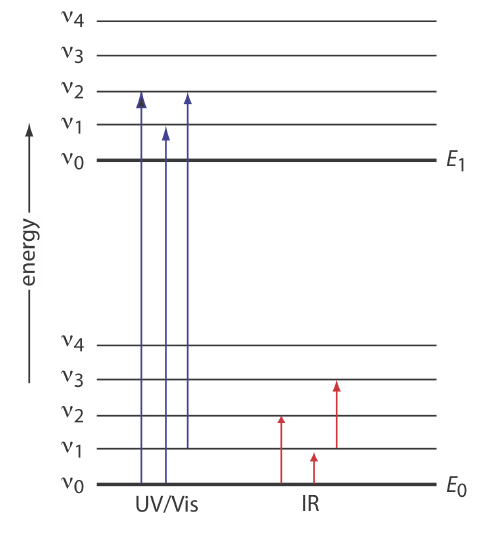
The types of energy states involved in emission and absorption depend on the energy of the electromagnetic radiation. In general, \(\gamma\)-rays involve transitions between nuclear states, X-rays probe the energies of core-level electrons, ultraviolet-visible radiation probes the energies of valence electrons, infrared radiation provides information on vibrational energy states, microwave radiation probes rotational energy levels and electron spins, and radio waves provide information on nuclear spins. While infrared spectroscopy may provide information on a molecule's vibrational energy states, the energies available in ultraviolet-visible spectroscopy provide information on both the molecule's electronic states and its vibrational states, as shown in Figure \(\PageIndex{5}\).

Figure \(\PageIndex{5}\). Diagram showing two electronic energy levels (E₀ and E₁), each with five vibrational energy levels \(\nu_{0-4}\). Absorption of ultraviolet and visible radiation (shown by the blue arrows) leads to a change in the analyte’s electronic energy levels and, possibly, a change in vibrational energy as well. A change in vibrational energy without a change in electronic energy levels occurs with the absorption of infrared radiation (shown by the red arrows).