6.2: Wave Properties of Electromagnetic Radiation

Ways to Characterize a Wave

Electromagnetic radiation consists of oscillating electric and magnetic fields that propagate through space along a linear path and with a constant velocity. The oscillations in the electric field and the magnetic field are perpendicular to each other and to the direction of the wave’s propagation. Figure \(\PageIndex{1}\) shows an example of plane-polarized electromagnetic radiation, which consists of a single oscillating electric field and a single oscillating magnetic field.

Figure \(\PageIndex{1}\). Plane-polarized electromagnetic radiation showing the oscillating electric field in blue and the oscillating magnetic field in red. The radiation’s amplitude, A, and its wavelength, \(\lambda\), are shown. Normally, electromagnetic radiation is unpolarized, with oscillating electric and magnetic fields present in all possible planes perpendicular to the direction of propagation.

Measurable Properties

An electromagnetic wave is characterized by several fundamental properties, including its velocity, amplitude, frequency, phase angle, polarization, and direction of propagation [Ball, D. W. Spectroscopy 1994, 9(5), 24–25]. Focusing on the oscillations in the electric field, amplitude is the maximum displacement of the electrical field. The wave's frequency, \(\nu\), is the number of oscillations in the electric field per unit time. Wavelength, \(\lambda\) is defined as the distance between successive maxima . Figure \(\PageIndex{1}\) shows the initial amplitude as 0; the phase angle \(\Phi\) accounts for the fact that the initial amplitude need not be zero, which we can accomplish by shifting the wave along the direction of propagation.

There is a relationship between wavelength and frequency, which is

\[\lambda = \frac {c} {\nu} \nonumber \]

where \(c\) is the speed of light in a vacuum. Another unit useful unit is the wavenumber, \(\overline{\nu}\), which is the reciprocal of the wavelength

\[\overline{\nu} = \frac {1} {\lambda} \nonumber \]

Wavenumbers frequently are used to characterize infrared radiation, with the units given in cm^–1. Power, \(P\), and intensity, \(I\), are two additional properties of light, both related to the square of the amplitude; power is the energy transferred per second and intensity is the power transferred to a given area.

In a vacuum, electromagnetic radiation travels at the speed of light, c, which is \(2.99792 \times 10^8\) m/s. When electromagnetic radiation moves through a medium other than a vacuum, its velocity, v, is less than the speed of light in a vacuum. The difference between v and c is sufficiently small (<0.1%) that the speed of light to three significant figures, \(3.00 \times 10^8\) m/s, is accurate enough for most purposes.

When electromagnetic radiation moves between different media—for example, when it moves from air into water—its frequency, \(\nu\), remains constant. Because its velocity depends upon the medium in which it is traveling, the electromagnetic radiation’s wavelength, \(\lambda\), changes. If we replace the speed of light in a vacuum, c, with its speed in the medium, \(v\), then the wavelength is

\[\lambda = \frac {v} {\nu} \nonumber \]

This change in wavelength as light passes between two media explains the refraction of electromagnetic radiation seen in the photograph of light passing through rain drop, what was included in the previous section. This is discussed in more detail later in this section.

Example 6.2.1

In 1817, Josef Fraunhofer studied the spectrum of solar radiation, observing a continuous spectrum with numerous dark lines. Fraunhofer labeled the most prominent of the dark lines with letters. In 1859, Gustav Kirchhoff showed that the D line in the sun’s spectrum was due to the absorption of solar radiation by sodium atoms. The wavelength of the sodium D line is 589 nm. What are the frequency and the wavenumber for this line?

Solution

The frequency and wavenumber of the sodium D line are

\[\nu=\frac{c}{\lambda}=\frac{3.00 \times 10^{8} \ \mathrm{m} / \mathrm{s}}{589 \times 10^{-9} \ \mathrm{m}}=5.09 \times 10^{14} \ \mathrm{s}^{-1} \nonumber \]

\[\overline{\nu}=\frac{1}{\lambda}=\frac{1}{589 \times 10^{-9} \ \mathrm{m}} \times \frac{1 \ \mathrm{m}}{100 \ \mathrm{cm}}=1.70 \times 10^{4} \ \mathrm{cm}^{-1} \nonumber \]

Exercise 6.2.1

Another historically important series of spectral lines is the Balmer series of emission lines from hydrogen. One of its lines has a wavelength of 656.3 nm. What are the frequency and the wavenumber for this line?

Answer

The frequency and wavenumber for the line are

\[\nu=\frac{c}{\lambda}=\frac{3.00 \times 10^{8} \ \mathrm{m} / \mathrm{s}}{656.3 \times 10^{-9} \ \mathrm{m}}=4.57 \times 10^{14} \ \mathrm{s}^{-1} \nonumber \]

\[\overline{\nu}=\frac{1}{\lambda}=\frac{1}{656.3 \times 10^{-9} \ \mathrm{m}} \times \frac{1 \ \mathrm{m}}{100 \ \mathrm{cm}}=1.524 \times 10^{4} \ \mathrm{cm}^{-1} \nonumber \]

Polarization

Figure \(\PageIndex{1}\) shows a single oscillating electrical field and, perpendicular to that, a single oscillating magnetic field. This is an example of plane polarized light in which oscillation of the electrical field occurs at just one angle. Normally electromagnetic radiation oscillates simultaneously at all possible angles. Figure \(\PageIndex{2}\) shows the difference in these two cases. If we observe the plane polarized light as it oscillates toward us, we see the single line at the top of the figure where blue indicates a positive amplitude and red indicates a negative amplitude, and where the opacity of the shading shows the change in the amplitudes. The vertical dashed lines show nodes where the amplitude is zero and where no light is seen. With ordinary light, we see a circular beam of radiation because the electrical field is oscillating at all angles. The amplitude's sign and magnitude, and the presence of nodes where the amplitude is zero, remain evident to us. Note that if we observe the source's intensity, then the each of the lines and circles in Figure \(\PageIndex{2}\) will appear blue (positive values as intensity is proportion to the square of the amplitude); we continue to observe fluctuations in the intensity and the presence of the nodes.

Figure \(\PageIndex{2}\): Illustration showing the difference between plane polarized light (top) and ordinary light (bottom). Blue is used to show positive amplitudes and red is used to show negative amplitudes. The opacity of the colors—which have values of 100%, 67%, 33%, and 0%—indicate the relative magnitudes of the amplitudes. When the opacity is 0%, the amplitude is zero and there is a node.

Mathematical Representation of Waves

We can describe the oscillations in the electric field as a sine wave

\[A_{t}=A_{e} \sin (2 \pi \nu t+\Phi) \nonumber \]

where A_t is the magnitude of the electric field at time t, A_e is the field’s maximum amplitude, \(\nu\) is the wave's frequency, and \(\Phi\) is a phase angle that accounts for the fact that \(A_t\) need not have a value of zero at time \(t = 0\). The identical equation for the magnetic field is

\[A_{t}=A_{m} \sin (2 \pi \nu t+\Phi) \nonumber \]

where A_m is the magnetic field’s maximum amplitude.

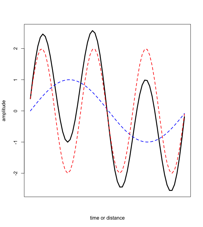
One of the important features of waves is that adding or subtracting together two (or more) gives a new wave. Figure \(\PageIndex{3}\) shows one example. The superposition of waves explains why two identical waves that are completely out-of-phase with each other produce a signal in which the amplitude is zero at all points.

Figure \(\PageIndex{3}\): Illustration of the principle of superposition. The x-axis scale runs from zero to \(2 \pi\). The equation for the wave shown as a dashed blue line is \(y = sin(x)\) and the equation for the wave shown as a dashed red line is \(y = 2 sin(\pi /16 + 3x)\). The sum of these two waves is the solid black line.

Another important consequence of the superposition of waves is that if we can add together a series of waves to produce a new wave, then there is a corresponding mathematical process that takes a complex wave and determines the underlying set of sine waves of which it is comprised. This process is called a Fourier transform, which we will revisit in later chapters.

Interactions of Waves With Matter

When light encounters matter—perhaps a particle, a solution, or a thin film—it can interact with it in several ways. In this section we consider two such interactions: refraction and reflection. Three additional types of interactions—the scattering of light, the diffraction of light, and the transmission of light—are considered in later chapters where they play an important role in specific instrumental methods of analysis.

Refraction

When light passes from one medium (perhaps air) into another medium (perhaps water) that has a different density, the light experiences a change in direction that is a consequence of a difference in its velocity in the two media. This bending of light is called refraction, the extent of which is given by Snell's law

\[ \frac{\text{sin } \theta_1} {\text{sin } \theta_2} = \frac {\eta_2} {\eta_1} = \frac {v_1} {v_2} \nonumber \]

where \(\eta_i\) is the refractive index of a medium and \(v_i\) is the velocity in a medium, and where the angles, \(\theta_i\), are shown in Figure \(\PageIndex{4}\).

Figure \(\PageIndex{4}\): Illustration of the refraction of light as it moves across the interface of two media with different refractive indexes. The angles of the light are given by \(\theta\) and are measured relative to a surface normal, which is shown by the dashed line. The denser medium has the smaller value of \(\theta\) and the larger the refractive index.

Reflection

In addition to refraction, when light crosses an interface that separates media with different refractive indexes, some of the light is reflected back. When then angle of incidence is 0° (that is, the light is perpendicular to the interface), then the fraction of light that is reflected is given by

\[\frac{I_r}{I_0} = \frac{(\eta_2 - \eta_1)^2}{(\eta_2 + \eta_1)^2} \nonumber \]

where \(I_r\) is the intensity of light that is reflected, \(I_0\) is the intensity of light from the source that enters the interface, and \(\eta_i\) is the refractive index of the media. If light crosses more than one interface—as is the case when light passes through a sample cell—then the total fraction of reflected light is the sum of the fraction of light reflected at each interface.