
10.8: Spectroscopy Based on Scattering
- Page ID
- 157679

\( \newcommand{\vecs}[1]{\overset { \scriptstyle \rightharpoonup} {\mathbf{#1}} } \)
\( \newcommand{\vecd}[1]{\overset{-\!-\!\rightharpoonup}{\vphantom{a}\smash {#1}}} \)
\( \newcommand{\dsum}{\displaystyle\sum\limits} \)
\( \newcommand{\dint}{\displaystyle\int\limits} \)
\( \newcommand{\dlim}{\displaystyle\lim\limits} \)
\( \newcommand{\id}{\mathrm{id}}\) \( \newcommand{\Span}{\mathrm{span}}\)
( \newcommand{\kernel}{\mathrm{null}\,}\) \( \newcommand{\range}{\mathrm{range}\,}\)
\( \newcommand{\RealPart}{\mathrm{Re}}\) \( \newcommand{\ImaginaryPart}{\mathrm{Im}}\)
\( \newcommand{\Argument}{\mathrm{Arg}}\) \( \newcommand{\norm}[1]{\| #1 \|}\)
\( \newcommand{\inner}[2]{\langle #1, #2 \rangle}\)
\( \newcommand{\Span}{\mathrm{span}}\)
\( \newcommand{\id}{\mathrm{id}}\)
\( \newcommand{\Span}{\mathrm{span}}\)
\( \newcommand{\kernel}{\mathrm{null}\,}\)
\( \newcommand{\range}{\mathrm{range}\,}\)
\( \newcommand{\RealPart}{\mathrm{Re}}\)
\( \newcommand{\ImaginaryPart}{\mathrm{Im}}\)
\( \newcommand{\Argument}{\mathrm{Arg}}\)
\( \newcommand{\norm}[1]{\| #1 \|}\)
\( \newcommand{\inner}[2]{\langle #1, #2 \rangle}\)
\( \newcommand{\Span}{\mathrm{span}}\) \( \newcommand{\AA}{\unicode[.8,0]{x212B}}\)
\( \newcommand{\vectorA}[1]{\vec{#1}} % arrow\)
\( \newcommand{\vectorAt}[1]{\vec{\text{#1}}} % arrow\)
\( \newcommand{\vectorB}[1]{\overset { \scriptstyle \rightharpoonup} {\mathbf{#1}} } \)
\( \newcommand{\vectorC}[1]{\textbf{#1}} \)
\( \newcommand{\vectorD}[1]{\overrightarrow{#1}} \)
\( \newcommand{\vectorDt}[1]{\overrightarrow{\text{#1}}} \)
\( \newcommand{\vectE}[1]{\overset{-\!-\!\rightharpoonup}{\vphantom{a}\smash{\mathbf {#1}}}} \)
\( \newcommand{\vecs}[1]{\overset { \scriptstyle \rightharpoonup} {\mathbf{#1}} } \)
\(\newcommand{\longvect}{\overrightarrow}\)
\( \newcommand{\vecd}[1]{\overset{-\!-\!\rightharpoonup}{\vphantom{a}\smash {#1}}} \)
\(\newcommand{\avec}{\mathbf a}\) \(\newcommand{\bvec}{\mathbf b}\) \(\newcommand{\cvec}{\mathbf c}\) \(\newcommand{\dvec}{\mathbf d}\) \(\newcommand{\dtil}{\widetilde{\mathbf d}}\) \(\newcommand{\evec}{\mathbf e}\) \(\newcommand{\fvec}{\mathbf f}\) \(\newcommand{\nvec}{\mathbf n}\) \(\newcommand{\pvec}{\mathbf p}\) \(\newcommand{\qvec}{\mathbf q}\) \(\newcommand{\svec}{\mathbf s}\) \(\newcommand{\tvec}{\mathbf t}\) \(\newcommand{\uvec}{\mathbf u}\) \(\newcommand{\vvec}{\mathbf v}\) \(\newcommand{\wvec}{\mathbf w}\) \(\newcommand{\xvec}{\mathbf x}\) \(\newcommand{\yvec}{\mathbf y}\) \(\newcommand{\zvec}{\mathbf z}\) \(\newcommand{\rvec}{\mathbf r}\) \(\newcommand{\mvec}{\mathbf m}\) \(\newcommand{\zerovec}{\mathbf 0}\) \(\newcommand{\onevec}{\mathbf 1}\) \(\newcommand{\real}{\mathbb R}\) \(\newcommand{\twovec}[2]{\left[\begin{array}{r}#1 \\ #2 \end{array}\right]}\) \(\newcommand{\ctwovec}[2]{\left[\begin{array}{c}#1 \\ #2 \end{array}\right]}\) \(\newcommand{\threevec}[3]{\left[\begin{array}{r}#1 \\ #2 \\ #3 \end{array}\right]}\) \(\newcommand{\cthreevec}[3]{\left[\begin{array}{c}#1 \\ #2 \\ #3 \end{array}\right]}\) \(\newcommand{\fourvec}[4]{\left[\begin{array}{r}#1 \\ #2 \\ #3 \\ #4 \end{array}\right]}\) \(\newcommand{\cfourvec}[4]{\left[\begin{array}{c}#1 \\ #2 \\ #3 \\ #4 \end{array}\right]}\) \(\newcommand{\fivevec}[5]{\left[\begin{array}{r}#1 \\ #2 \\ #3 \\ #4 \\ #5 \\ \end{array}\right]}\) \(\newcommand{\cfivevec}[5]{\left[\begin{array}{c}#1 \\ #2 \\ #3 \\ #4 \\ #5 \\ \end{array}\right]}\) \(\newcommand{\mattwo}[4]{\left[\begin{array}{rr}#1 \amp #2 \\ #3 \amp #4 \\ \end{array}\right]}\) \(\newcommand{\laspan}[1]{\text{Span}\{#1\}}\) \(\newcommand{\bcal}{\cal B}\) \(\newcommand{\ccal}{\cal C}\) \(\newcommand{\scal}{\cal S}\) \(\newcommand{\wcal}{\cal W}\) \(\newcommand{\ecal}{\cal E}\) \(\newcommand{\coords}[2]{\left\{#1\right\}_{#2}}\) \(\newcommand{\gray}[1]{\color{gray}{#1}}\) \(\newcommand{\lgray}[1]{\color{lightgray}{#1}}\) \(\newcommand{\rank}{\operatorname{rank}}\) \(\newcommand{\row}{\text{Row}}\) \(\newcommand{\col}{\text{Col}}\) \(\renewcommand{\row}{\text{Row}}\) \(\newcommand{\nul}{\text{Nul}}\) \(\newcommand{\var}{\text{Var}}\) \(\newcommand{\corr}{\text{corr}}\) \(\newcommand{\len}[1]{\left|#1\right|}\) \(\newcommand{\bbar}{\overline{\bvec}}\) \(\newcommand{\bhat}{\widehat{\bvec}}\) \(\newcommand{\bperp}{\bvec^\perp}\) \(\newcommand{\xhat}{\widehat{\xvec}}\) \(\newcommand{\vhat}{\widehat{\vvec}}\) \(\newcommand{\uhat}{\widehat{\uvec}}\) \(\newcommand{\what}{\widehat{\wvec}}\) \(\newcommand{\Sighat}{\widehat{\Sigma}}\) \(\newcommand{\lt}{<}\) \(\newcommand{\gt}{>}\) \(\newcommand{\amp}{&}\) \(\definecolor{fillinmathshade}{gray}{0.9}\)The blue color of the sky during the day and the red color of the sun at sunset are the result of light scattered by small particles of dust, molecules of water, and other gases in the atmosphere. The efficiency of a photon’s scattering depends on its wavelength. We see the sky as blue during the day because violet and blue light scatter to a greater extent than other, longer wavelengths of light. For the same reason, the sun appears red at sunset because red light is less efficiently scattered and is more likely to pass through the atmosphere than other wavelengths of light. The scattering of radiation has been studied since the late 1800s, with applications beginning soon thereafter. The earliest quantitative applications of scattering, which date from the early 1900s, used the elastic scattering of light by colloidal suspensions to determine the concentration of colloidal particles.
Origin of Scattering
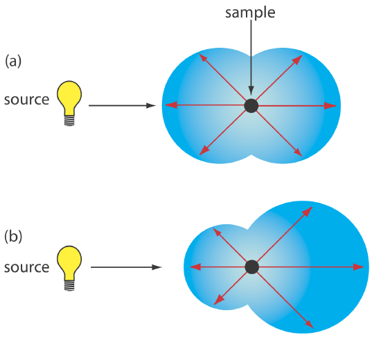
If we send a focused, monochromatic beam of radiation with a wavelength \(\lambda\) through a medium of particles with dimensions \(< 1.5 \lambda\), the radiation scatters in all directions. For example, visible radiation of 500 nm is scattered by particles as large as 750 nm in the longest dimension. Two general categories of scattering are recognized. In elastic scattering, radiation is first absorbed by the particles and then emitted without undergoing a change in the radiation’s energy. When the radiation emerges with a change in energy, the scattering is inelastic. Only elastic scattering is considered in this text.
Elastic scattering is divided into two types: Rayleigh, or small-particle scattering, and large-particle scattering. Rayleigh scattering occurs when the scattering particle’s largest dimension is less than 5% of the radiation’s wavelength. The intensity of the scattered radiation is proportional to its frequency to the fourth power, \(\nu^4\)—which accounts for the greater scattering of blue light than red light—and is distributed symmetrically (Figure 10.8.1 a). For larger particles, scattering increases in the forward direction and decreases in the backward direction as the result of constructive and destructive interferences (Figure 10.8.1 b).
Turbidimetry and Nephelometry
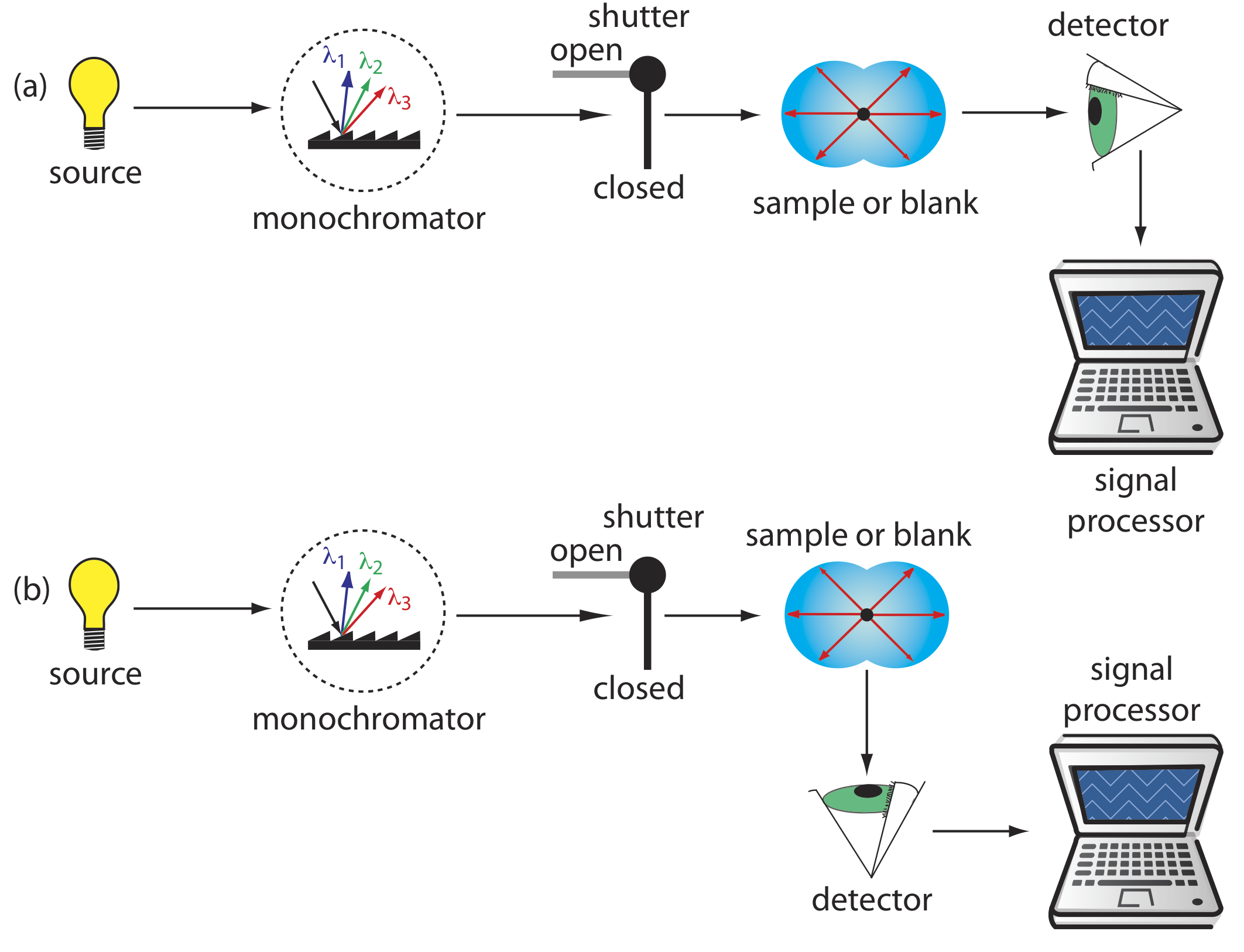
Turbidimetry and nephelometry are two techniques that rely on the elastic scattering of radiation by a suspension of colloidal particles. In turbidimetry the detector is placed in line with the source and the decrease in the radiation’s transmitted power is measured. In nephelometry the scattered radiation is measured at an angle of 90o to the source. The similarity of turbidimetry to absorbance spectroscopy and of nephelometry to fluorescence spectroscopy is evident in the instrumental designs shown in Figure 10.8.2 . In fact, we can use a UV/Vis spectrophotometer for turbidimetry and we can use a spectrofluorometer for nephelometry.
Turbidimetry or Nephelometry?
When developing a scattering method the choice between using turbidimetry or using nephelometry is determined by two factors. The most important consideration is the intensity of the scattered radiation relative to the intensity of the source’s radiation. If the solution contains a small concentration of scattering particles, then the intensity of the transmitted radiation, IT, is approximately the same as the intensity of the source’s radiation, I0. As we learned earlier in the section on molecular absorption, there is substantial uncertainty in determining a small difference between two intense signals. For this reason, nephelometry is a more appropriate choice for a sample that contains few scattering particles. Turbidimetry is a better choice when the sample contains a high concentration of scattering particles.
A second consideration in choosing between turbidimetry and nephelometry is the size of the scattering particles. For nephelometry, the intensity of scattered radiation at 90o increases when the particles are small and Rayleigh scattering is in effect. For larger particles, as shown in Figure 10.8.1 , the intensity of scattering decreases at 90o. When using an ultraviolet or a visible source of radiation, the optimum particle size is 0.1–1 μm. The size of the scattering particles is less important for turbidimetry where the signal is the relative decrease in transmitted radiation. In fact, turbidimetric measurements are feasible even when the size of the scattering particles results in an increase in reflection and refraction, although a linear relationship between the signal and the concentration of scattering particles may no longer hold.
Determining Concentration by Turbidimetry
For turbidimetry the measured transmittance, T, is the ratio of the intensity of source radiation transmitted by the sample, IT, to the intensity of source radiation transmitted by a blank, I0.
\[T=\frac{I_{\mathrm{T}}}{I_{0}} \nonumber\]
The relationship between transmittance and the concentration of the scattering particles is similar to that given by Beer’s law
\[-\log T=k b C \label{10.1}\]
where C is the concentration of the scattering particles in mass per unit volume (w/v), b is the pathlength, and k is a constant that depends on several factors, including the size and shape of the scattering particles and the wavelength of the source radiation. The exact relationship is established by a calibration curve prepared using a series of standards that contain known concentrations of analyte. As with Beer’s law, Equation \ref{10.1} may show appreciable deviations from linearity.
Determining Concentration by Nephelometry
For nephelometry the relationship between the intensity of scattered radiation, IS, and the concentration of scattering particles is
\[I_{\mathrm{s}}=k I_{0} C \label{10.2}\]
where k is an empirical constant for the system and I0 is the intensity of the source radiation. The value of k is determined from a calibration curve prepared using a series of standards that contain known concentrations of analyte.
Selecting a Wavelength for the Incident Radiation
The choice of wavelength is based primarily on the need to minimize potential interferences. For turbidimetry, where the incident radiation is transmitted through the sample, a monochromator or filter allow us to avoid wavelengths that are absorbed instead of scattered by the sample. For nephelometry, the absorption of incident radiation is not a problem unless it induces fluorescence from the sample. With a nonfluorescent sample there is no need for wavelength selection and a source of white light may be used as the incident radiation. For both techniques, other considerations in choosing a wavelength including the intensity of scattering, the trans- ducer’s sensitivity (many common photon transducers are more sensitive to radiation at 400 nm than at 600 nm), and the source’s intensity.
Preparing the Sample for Analysis
Although Equation \ref{10.1} and Equation \ref{10.2} relate scattering to the concentration of the scattering particles, the intensity of scattered radiation also is influenced by the size and the shape of the scattering particles. Samples that contain the same number of scattering particles may show significantly different values for –logT or IS depending on the average diameter of the particles. For a quantitative analysis, therefore, it is necessary to maintain a uniform distribution of particle sizes throughout the sample and between samples and standards.
Most turbidimetric and nephelometric methods rely on precipitation reaction to form the scattering particles. As we learned in Chapter 8, a precipitate’s properties, including particle size, are determined by the conditions under which it forms. To maintain a reproducible distribution of particle sizes between samples and standards, it is necessary to control parameters such as the concentration of reagents, the order of adding reagents, the pH and temperature, the agitation or stirring rate, the ionic strength, and the time between the precipitate’s initial formation and the measurement of transmittance or scattering. In many cases a surface-active agent—such as glycerol, gelatin, or dextrin—is added to stabilize the precipitate in a colloidal state and to prevent the coagulation of the particles.
Applications
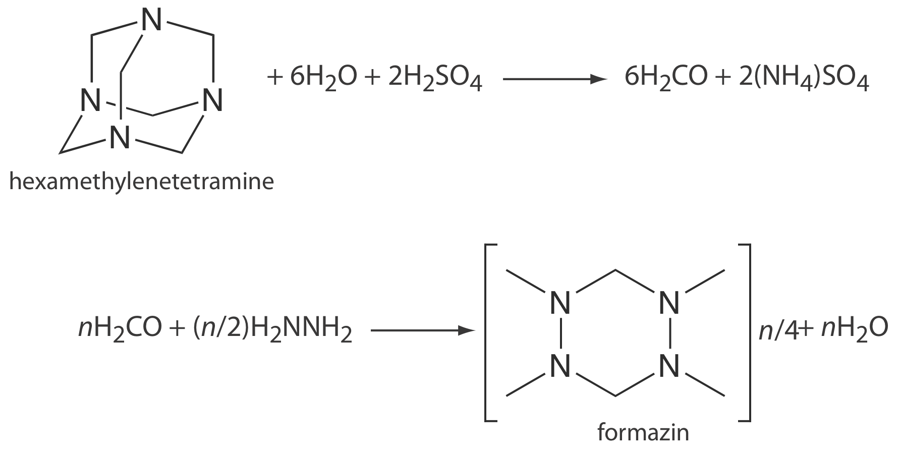
Turbidimetry and nephelometry are used to determine the clarity of water. The primary standard for measuring clarity is formazin, an easily prepared, stable polymer suspension (Figure 10.8.3 ) [Hach, C. C.; Bryant, M. “Turbidity Standards,” Technical Information Series, Booklet No. 12, Hach Company: Loveland, CO, 1995]. A stock standard of formazin is prepared by combining a 1g/100mL solution of hydrazine sulfate, N2H4•H2SO4, with a 10 g/100 mL solution of hexamethylenetetramine to produce a suspension of particles that is defined as 4000 nephelometric turbidity units (NTU). A set of external standards with NTUs between 0 and 40 is prepared by diluting the stock standard. This method is readily adapted to the analysis of the clarity of orange juice, beer, and maple syrup.
A number of inorganic cations and anions are determined by precipitating them under well-defined conditions. The transmittance or scattering of light, as defined by Equation \ref{10.1} or Equation \ref{10.2}, is proportional to the concentration of the scattering particles, which, in turn, is related by the stoichiometry of the precipitation reaction to the analyte’s concentration. Several examples of analytes determined in this way are listed in Table 10.8.1 .
Representative Method 10.8.1: Turbidimetric Determination of Sulfate in Water
The best way to appreciate the theoretical and the practical details discussed in this section is to carefully examine a typical analytical method. Although each method is unique, the following description of the determination of sulfate in water provides an instructive example of a typical procedure. The description here is based on Method 4500–SO42––C in Standard Methods for the Analysis of Water and Wastewater, American Public Health Association: Washington, D. C. 20th Ed., 1998.
Description of Method
Adding BaCl2 to an acidified sample precipitates \(\text{SO}_4^{2-}\) as BaSO4. The concentration of \(\text{SO}_4^{2-}\) is determined either by turbidimetry or by nephelometry using an incident source of radiation of 420 nm. External standards that contain know concentrations of \(\text{SO}_4^{2-}\) are used to standardize the method.
Procedure
Transfer a 100-mL sample to a 250-mL Erlenmeyer flask along with 20.00 mL of an appropriate buffer. For a sample that contains more than 10 mg \(\text{SO}_4^{2-}\)/L, the buffer’s composition is 30 g of MgCl2•6H2O, 5 g of CH3COONa•3H2O, 1.0 g of KNO3, and 20 mL of glacial CH3COOH per liter. The buffer for a sample that contain less than 10 mg \(\text{SO}_4^{2-}\)/L is the same except for the addition of 0.111 g of Na2SO4 per L.
Place the sample and the buffer on a magnetic stirrer operated at the same speed for all samples and standards. Add a spoonful of 20–30 mesh BaCl2, using a measuring spoon with a capacity of 0.2–0.3 mL, to precipitate the \(\text{SO}_4^{2-}\) as BaSO4. Begin timing when the BaCl2 is added and stir the suspension for 60 ± 2 s. When the stirring is complete, allow the solution to sit without stirring for 5.0± 0.5 min before measuring its transmittance or its scattering.
Prepare a calibration curve over the range 0–40 mg \(\text{SO}_4^{2-}\)/L by diluting a stock standard that is 100-mg \(\text{SO}_4^{2-}\)/L. Treat each standard using the procedure described above for the sample. Prepare a calibration curve and use it to determine the amount of sulfate in the sample.
Questions
1. What is the purpose of the buffer?
If the precipitate’s particles are too small, IT is too small to measure reliably. Because rapid precipitation favors the formation of micro-crystalline particles of BaSO4, we use conditions that favor the precipitate’s growth over the nucleation of new particles. The buffer’s high ionic strength and its acidity favor the precipitate’s growth and prevent the formation of microcrystalline BaSO4.
2. Why is it important to use the same stirring rate and time for the samples and standards?
How fast and how long we stir the sample after we add BaCl2 influences the size of the precipitate’s particles.
3. Many natural waters have a slight color due to the presence of humic and fulvic acids, and may contain suspended matter (Figure 10.8.4 ). Explain why these might interfere with the analysis for sulfate. For each interferent, suggest a way to minimize its effect on the analysis.
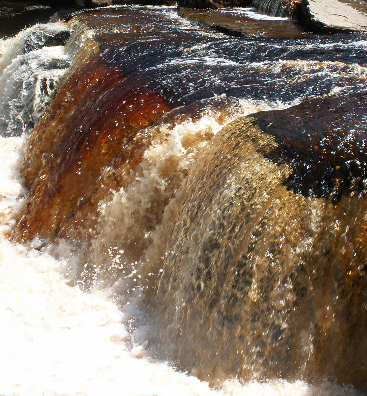
Suspended matter in a sample contributes to scattering and, therefore, results in a positive determinate error. We can eliminate this interference by filtering the sample prior to its analysis. A sample that is colored may absorb some of the source’s radiation, leading to a positive determinate error. We can compensate for this interference by taking a sample through the analysis without adding BaCl2. Because no precipitate forms, we use the transmittance of this sample blank to correct for the interference.
4. Why is Na2SO4 added to the buffer for samples that contain less than 10 mg \(\text{SO}_4^{2-}\)/L?
The uncertainty in a calibration curve is smallest near its center. If a sample has a high concentration of \(\text{SO}_4^{2-}\), we can dilute it so that its concentration falls near the middle of the calibration curve. For a sample with a small concentration of \(\text{SO}_4^{2-}\), the buffer increases the concentration of sulfate by
\[\begin{array}{c}{\frac{0.111 \ \mathrm{g} \ \mathrm{Na}_{2} \mathrm{SO}_{4}}{\mathrm{L}} \times \frac{96.06 \ \mathrm{g} \ \mathrm{SO}_{4}^{2-}}{142.04 \ \mathrm{g} \ \mathrm{Na}_{2} \mathrm{SO}_{4}} \times} \\ {\qquad \frac{1000 \ \mathrm{mg}}{\mathrm{g}} \times \frac{20.00 \ \mathrm{mL}}{250.0 \ \mathrm{mL}}=6.00 \ \mathrm{mg} \ \mathrm{SO}_{4}^{2-} / \mathrm{L}}\end{array} \nonumber\]
After using the calibration curve to determine the amount of sulfate in the sample as analyzed, we subtract 6.00 mg \(\text{SO}_4^{2-}\)/L to determine the amount of sulfate in the original sample.
To evaluate the method described in Representative Method 10.8.1, a series of external standard was prepared and analyzed, providing the results shown in the following table.
| mg \(\text{SO}_4^{2-}\)/L | transmittance |
|---|---|
| 0.00 | 1.00 |
| 10.00 | 0.646 |
| 20.00 | 0.417 |
| 30.00 | 0.269 |
| 40.00 | 0.174 |
Analysis of a 100.0-mL sample of a surface water gives a transmittance of 0.538. What is the concentration of sulfate in the sample?
Solution
Linear regression of –logT versus concentration of \(\text{SO}_4^{2-}\) gives the calibration curve shown below, which has the following calibration equation.
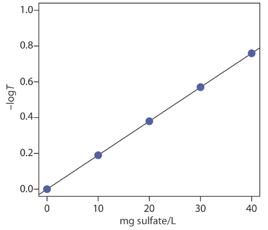
\[-\log T=-1.04 \times 10^{-5}+0.0190 \times \frac{\mathrm{mg} \ \mathrm{SO}_{4}^{2-}}{\mathrm{L}} \nonumber\]
Substituting the sample’s transmittance into the calibration curve’s equation gives the concentration of sulfate in sample as 14.2 mg \(\text{SO}_4^{2-}\)/L.