
10.7: Atomic Emission Spectroscopy
- Page ID
- 157678

\( \newcommand{\vecs}[1]{\overset { \scriptstyle \rightharpoonup} {\mathbf{#1}} } \)
\( \newcommand{\vecd}[1]{\overset{-\!-\!\rightharpoonup}{\vphantom{a}\smash {#1}}} \)
\( \newcommand{\dsum}{\displaystyle\sum\limits} \)
\( \newcommand{\dint}{\displaystyle\int\limits} \)
\( \newcommand{\dlim}{\displaystyle\lim\limits} \)
\( \newcommand{\id}{\mathrm{id}}\) \( \newcommand{\Span}{\mathrm{span}}\)
( \newcommand{\kernel}{\mathrm{null}\,}\) \( \newcommand{\range}{\mathrm{range}\,}\)
\( \newcommand{\RealPart}{\mathrm{Re}}\) \( \newcommand{\ImaginaryPart}{\mathrm{Im}}\)
\( \newcommand{\Argument}{\mathrm{Arg}}\) \( \newcommand{\norm}[1]{\| #1 \|}\)
\( \newcommand{\inner}[2]{\langle #1, #2 \rangle}\)
\( \newcommand{\Span}{\mathrm{span}}\)
\( \newcommand{\id}{\mathrm{id}}\)
\( \newcommand{\Span}{\mathrm{span}}\)
\( \newcommand{\kernel}{\mathrm{null}\,}\)
\( \newcommand{\range}{\mathrm{range}\,}\)
\( \newcommand{\RealPart}{\mathrm{Re}}\)
\( \newcommand{\ImaginaryPart}{\mathrm{Im}}\)
\( \newcommand{\Argument}{\mathrm{Arg}}\)
\( \newcommand{\norm}[1]{\| #1 \|}\)
\( \newcommand{\inner}[2]{\langle #1, #2 \rangle}\)
\( \newcommand{\Span}{\mathrm{span}}\) \( \newcommand{\AA}{\unicode[.8,0]{x212B}}\)
\( \newcommand{\vectorA}[1]{\vec{#1}} % arrow\)
\( \newcommand{\vectorAt}[1]{\vec{\text{#1}}} % arrow\)
\( \newcommand{\vectorB}[1]{\overset { \scriptstyle \rightharpoonup} {\mathbf{#1}} } \)
\( \newcommand{\vectorC}[1]{\textbf{#1}} \)
\( \newcommand{\vectorD}[1]{\overrightarrow{#1}} \)
\( \newcommand{\vectorDt}[1]{\overrightarrow{\text{#1}}} \)
\( \newcommand{\vectE}[1]{\overset{-\!-\!\rightharpoonup}{\vphantom{a}\smash{\mathbf {#1}}}} \)
\( \newcommand{\vecs}[1]{\overset { \scriptstyle \rightharpoonup} {\mathbf{#1}} } \)
\(\newcommand{\longvect}{\overrightarrow}\)
\( \newcommand{\vecd}[1]{\overset{-\!-\!\rightharpoonup}{\vphantom{a}\smash {#1}}} \)
\(\newcommand{\avec}{\mathbf a}\) \(\newcommand{\bvec}{\mathbf b}\) \(\newcommand{\cvec}{\mathbf c}\) \(\newcommand{\dvec}{\mathbf d}\) \(\newcommand{\dtil}{\widetilde{\mathbf d}}\) \(\newcommand{\evec}{\mathbf e}\) \(\newcommand{\fvec}{\mathbf f}\) \(\newcommand{\nvec}{\mathbf n}\) \(\newcommand{\pvec}{\mathbf p}\) \(\newcommand{\qvec}{\mathbf q}\) \(\newcommand{\svec}{\mathbf s}\) \(\newcommand{\tvec}{\mathbf t}\) \(\newcommand{\uvec}{\mathbf u}\) \(\newcommand{\vvec}{\mathbf v}\) \(\newcommand{\wvec}{\mathbf w}\) \(\newcommand{\xvec}{\mathbf x}\) \(\newcommand{\yvec}{\mathbf y}\) \(\newcommand{\zvec}{\mathbf z}\) \(\newcommand{\rvec}{\mathbf r}\) \(\newcommand{\mvec}{\mathbf m}\) \(\newcommand{\zerovec}{\mathbf 0}\) \(\newcommand{\onevec}{\mathbf 1}\) \(\newcommand{\real}{\mathbb R}\) \(\newcommand{\twovec}[2]{\left[\begin{array}{r}#1 \\ #2 \end{array}\right]}\) \(\newcommand{\ctwovec}[2]{\left[\begin{array}{c}#1 \\ #2 \end{array}\right]}\) \(\newcommand{\threevec}[3]{\left[\begin{array}{r}#1 \\ #2 \\ #3 \end{array}\right]}\) \(\newcommand{\cthreevec}[3]{\left[\begin{array}{c}#1 \\ #2 \\ #3 \end{array}\right]}\) \(\newcommand{\fourvec}[4]{\left[\begin{array}{r}#1 \\ #2 \\ #3 \\ #4 \end{array}\right]}\) \(\newcommand{\cfourvec}[4]{\left[\begin{array}{c}#1 \\ #2 \\ #3 \\ #4 \end{array}\right]}\) \(\newcommand{\fivevec}[5]{\left[\begin{array}{r}#1 \\ #2 \\ #3 \\ #4 \\ #5 \\ \end{array}\right]}\) \(\newcommand{\cfivevec}[5]{\left[\begin{array}{c}#1 \\ #2 \\ #3 \\ #4 \\ #5 \\ \end{array}\right]}\) \(\newcommand{\mattwo}[4]{\left[\begin{array}{rr}#1 \amp #2 \\ #3 \amp #4 \\ \end{array}\right]}\) \(\newcommand{\laspan}[1]{\text{Span}\{#1\}}\) \(\newcommand{\bcal}{\cal B}\) \(\newcommand{\ccal}{\cal C}\) \(\newcommand{\scal}{\cal S}\) \(\newcommand{\wcal}{\cal W}\) \(\newcommand{\ecal}{\cal E}\) \(\newcommand{\coords}[2]{\left\{#1\right\}_{#2}}\) \(\newcommand{\gray}[1]{\color{gray}{#1}}\) \(\newcommand{\lgray}[1]{\color{lightgray}{#1}}\) \(\newcommand{\rank}{\operatorname{rank}}\) \(\newcommand{\row}{\text{Row}}\) \(\newcommand{\col}{\text{Col}}\) \(\renewcommand{\row}{\text{Row}}\) \(\newcommand{\nul}{\text{Nul}}\) \(\newcommand{\var}{\text{Var}}\) \(\newcommand{\corr}{\text{corr}}\) \(\newcommand{\len}[1]{\left|#1\right|}\) \(\newcommand{\bbar}{\overline{\bvec}}\) \(\newcommand{\bhat}{\widehat{\bvec}}\) \(\newcommand{\bperp}{\bvec^\perp}\) \(\newcommand{\xhat}{\widehat{\xvec}}\) \(\newcommand{\vhat}{\widehat{\vvec}}\) \(\newcommand{\uhat}{\widehat{\uvec}}\) \(\newcommand{\what}{\widehat{\wvec}}\) \(\newcommand{\Sighat}{\widehat{\Sigma}}\) \(\newcommand{\lt}{<}\) \(\newcommand{\gt}{>}\) \(\newcommand{\amp}{&}\) \(\definecolor{fillinmathshade}{gray}{0.9}\)The focus of this section is on the emission of ultraviolet and visible radiation following the thermal excitation of atoms. Atomic emission spectroscopy has a long history. Qualitative applications based on the color of flames were used in the smelting of ores as early as 1550 and were more fully developed around 1830 with the observation of atomic spectra generated by flame emission and spark emission [Dawson, J. B. J. Anal. At. Spectrosc. 1991, 6, 93–98]. Quantitative applications based on the atomic emission from electric sparks were developed by Lockyer in the early 1870 and quantitative applications based on flame emission were pioneered by Lundegardh in 1930. Atomic emission based on emission from a plasma was introduced in 1964.
For an on-line introduction to much of the material in this section, see Atomic Emission Spectroscopy (AES) by Tomas Spudich and Alexander Scheeline, a resource that is part of the Analytical Sciences Digital Library.
Atomic Emission Spectra
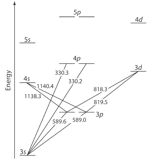
Atomic emission occurs when a valence electron in a higher energy atomic orbital returns to a lower energy atomic orbital. Figure 10.7.1 shows a portion of the energy level diagram for sodium, which consists of a series of discrete lines at wavelengths that correspond to the difference in energy between two atomic orbitals.
The intensity of an atomic emission line, Ie, is proportional to the number of atoms, \(N^*\), that populate the excited state,
where k is a constant that accounts for the efficiency of the transition. If a system of atoms is in thermal equilibrium, the population of excited state i is related to the total concentration of atoms, N, by the Boltzmann distribution. For many elements at temperatures of less than 5000 K the Boltzmann distribution is approximated as
\[N^* = N\left(\frac{g_{i}}{g_{0}}\right) e^{-E_i / k T} \label{10.2}\]
where gi and g0 are statistical factors that account for the number of equivalent energy levels for the excited state and the ground state, Ei is the energy of the excited state relative to a ground state energy, E0, k is Boltzmann’s constant (\(1.3807 \times 10^{-23}\) J/K), and T is the temperature in Kelvin. From Equation \ref{10.2} we expect that excited states with lower energies have larger populations and more intense emission lines. We also expect emission intensity to increase with temperature.
Equipment
An atomic emission spectrometer is similar in design to the instrumentation for atomic absorption. In fact, it is easy to adapt most flame atomic absorption spectrometers for atomic emission by turning off the hollow cathode lamp and monitoring the difference between the emission intensity when aspirating the sample and when aspirating a blank. Many atomic emission spectrometers, however, are dedicated instruments designed to take advantage of features unique to atomic emission, including the use of plasmas, arcs, sparks, and lasers as atomization and excitation sources, and an enhanced capability for multielemental analysis.
Atomization and Excitation
Atomic emission requires a means for converting into a free gaseous atom an analyte that is present in a solid, liquid, or solution sample. The same source of thermal energy used for atomization usually serves as the excitation source. The most common methods are flames and plasmas, both of which are useful for liquid or solution samples. Solid samples are analyzed by dissolving in a solvent and using a flame or plasma atomizer.
Flame Sources
Atomization and excitation in flame atomic emission is accomplished with the same nebulization and spray chamber assembly used in atomic absorption (Figure 10.4.1). The burner head consists of a single or multiple slots, or a Meker-style burner. Older atomic emission instruments often used a total consumption burner in which the sample is drawn through a capillary tube and injected directly into the flame.
A Meker burner is similar to the more common Bunsen burner found in most laboratories; it is designed to allow for higher temperatures and for a larger diameter flame.
Plasma Sources
A plasma is a hot, partially ionized gas that contains an abundant concentration of cations and electrons. The plasma used in atomic emission is formed by ionizing a flowing stream of argon gas, producing argon ions and electrons. A plasma’s high temperature results from resistive heating as the electrons and argon ions move through the gas. Because a plasma operates at a much higher temperature than a flame, it provides for a better atomization efficiency and a higher population of excited states.
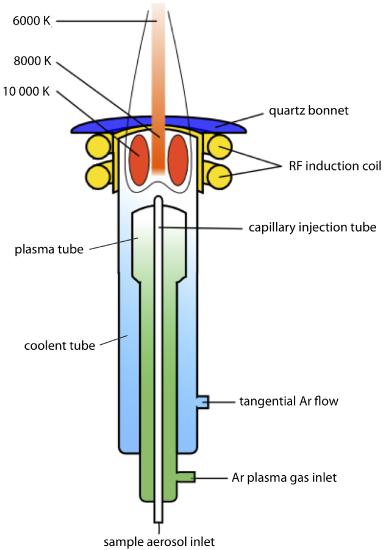
A schematic diagram of the inductively coupled plasma source (ICP) is shown in Figure 10.7.2 . The ICP torch consists of three concentric quartz tubes, surrounded at the top by a radio-frequency induction coil. The sample is mixed with a stream of Ar using a nebulizer, and is carried to the plasma through the torch’s central capillary tube. Plasma formation is initiated by a spark from a Tesla coil. An alternating radio-frequency current in the induction coil creates a fluctuating magnetic field that induces the argon ions and the electrons to move in a circular path. The resulting collisions with the abundant unionized gas give rise to resistive heating, providing temperatures as high as 10000 K at the base of the plasma, and between 6000 and 8000 K at a height of 15–20 mm above the coil, where emission usually is measured. At these high temperatures the outer quartz tube must be thermally isolated from the plasma. This is accomplished by the tangential flow of argon shown in the schematic diagram.
Multielemental Analysis
Atomic emission spectroscopy is ideally suited for a multielemental analysis because all analytes in a sample are excited simultaneously. If the instrument includes a scanning monochromator, we can program it to move rapidly to an analyte’s desired wavelength, pause to record its emission intensity, and then move to the next analyte’s wavelength. This sequential analysis allows for a sampling rate of 3–4 analytes per minute.
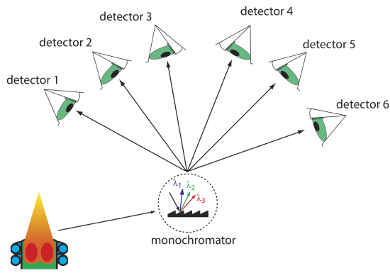
Another approach to a multielemental analysis is to use a multichannel instrument that allows us to monitor simultaneously many analytes. A simple design for a multichannel spectrometer, shown in Figure 10.7.3 , couples a monochromator with multiple detectors that are positioned in a semicircular array around the monochromator at positions that correspond to the wavelengths for the analytes.
Quantitative Applications
Atomic emission is used widely for the analysis of trace metals in a variety of sample matrices. The development of a quantitative atomic emission method requires several considerations, including choosing a source for atomization and excitation, selecting a wavelength and slit width, preparing the sample for analysis, minimizing spectral and chemical interferences, and selecting a method of standardization.
Choice of Atomization and Excitation Source
Except for the alkali metals, detection limits when using an ICP are significantly better than those obtained with flame emission (Table 10.7.1 ). Plasmas also are subject to fewer spectral and chemical interferences. For these reasons a plasma emission source is usually the better choice.
Selecting the Wavelength and Slit Width
The choice of wavelength is dictated by the need for sensitivity and the need to avoid interferences from the emission lines of other constituents in the sample. Because an analyte’s atomic emission spectrum has an abundance of emission lines—particularly when using a high temperature plasma source—it is inevitable that there will be some overlap between emission lines. For example, an analysis for Ni using the atomic emission line at 349.30 nm is complicated by the atomic emission line for Fe at 349.06 nm.
A narrower slit width provides better resolution, but at the cost of less radiation reaching the detector. The easiest approach to selecting a wavelength is to record the sample’s emission spectrum and look for an emission line that provides an intense signal and is resolved from other emission lines.
Preparing the Sample
Flame and plasma sources are best suited for samples in solution and in liquid form. Although a solid sample can be analyzed by directly inserting it into the flame or plasma, they usually are first brought into solution by digestion or extraction.
Minimizing Spectral Interferences
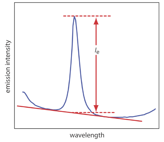
The most important spectral interference is broad, background emission from the flame or plasma and emission bands from molecular species. This background emission is particularly severe for flames because the temperature is insufficient to break down refractory compounds, such as oxides and hydroxides. Background corrections for flame emission are made by scanning over the emission line and drawing a baseline (Figure 10.7.4 ). Because a plasma’s temperature is much higher, a background interference due to molecular emission is less of a problem. Although emission from the plasma’s core is strong, it is insignificant at a height of 10–30 mm above the core where measurements normally are made.
Minimizing Chemical Interferences
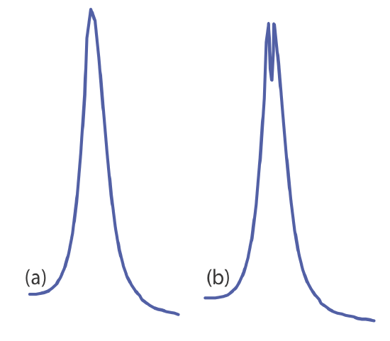
Flame emission is subject to the same types of chemical interferences as atomic absorption; they are minimized using the same methods: by adjusting the flame’s composition and by adding protecting agents, releasing agents, or ionization suppressors. An additional chemical interference results from self-absorption. Because the flame’s temperature is greatest at its center, the concentration of analyte atoms in an excited state is greater at the flame’s center than at its outer edges. If an excited state atom in the flame’s center emits a photon, then a ground state atom in the cooler, outer regions of the flame may absorb the photon, which decreases the emission intensity. For higher concentrations of analyte self-absorption may invert the center of the emission band (Figure 10.7.5 ).
Chemical interferences when using a plasma source generally are not significant because the plasma’s higher temperature limits the formation of nonvolatile species. For example, \(\text{PO}_4^{3-}\) is a significant interferent when analyzing samples for Ca2+ by flame emission, but has a negligible effect when using a plasma source. In addition, the high concentration of electrons from the ionization of argon minimizes ionization interferences.
Standardizing the Method
From Equation \ref{10.1} we know that emission intensity is proportional to the population of the analyte’s excited state, \(N^*\). If the flame or plasma is in thermal equilibrium, then the excited state population is proportional to the analyte’s total population, N, through the Boltzmann distribution (Equation \ref{10.2}).
A calibration curve for flame emission usually is linear over two to three orders of magnitude, with ionization limiting linearity when the analyte’s concentrations is small and self-absorption limiting linearity at higher concentrations of analyte. When using a plasma, which suffers from fewer chemical interferences, the calibration curve often is linear over four to five orders of magnitude and is not affected significantly by changes in the matrix of the standards.
Emission intensity is affected significantly by many parameters, including the temperature of the excitation source and the efficiency of atomization. An increase in temperature of 10 K, for example, produces a 4% increase in the fraction of Na atoms in the 3p excited state, an uncertainty in the signal that may limit the use of external standards. The method of internal standards is used when the variations in source parameters are difficult to control. To compensate for changes in the temperature of the excitation source, the internal standard is selected so that its emission line is close to the analyte’s emission line. In addition, the internal standard should be subject to the same chemical interferences to compensate for changes in atomization efficiency. To accurately correct for these errors the analyte and internal standard emission lines are monitored simultaneously.
Representative Method 10.7.1: Determination of Sodium in a Salt Substitute
The best way to appreciate the theoretical and the practical details discussed in this section is to carefully examine a typical analytical method. Although each method is unique, the following description of the determination of sodium in salt substitutes provides an instructive example of a typical procedure. The description here is based on Goodney, D. E. J. Chem. Educ. 1982, 59, 875–876.
Description of Method
Salt substitutes, which are used in place of table salt for individuals on low-sodium diets, replaces NaCl with KCl. Depending on the brand, fumaric acid, calcium hydrogen phosphate, or potassium tartrate also are present. Although intended to be sodium-free, salt substitutes contain small amounts of NaCl as an impurity. Typically, the concentration of sodium in a salt substitute is about 100 μg/g The exact concentration of sodium is determined by flame atomic emission. Because it is difficult to match the matrix of the standards to that of the sample, the analysis is accomplished by the method of standard additions.
Procedure
A sample is prepared by placing an approximately 10-g portion of the salt substitute in 10 mL of 3 M HCl and 100 mL of distilled water. After the sample has dissolved, it is transferred to a 250-mL volumetric flask and diluted to volume with distilled water. A series of standard additions is prepared by placing 25-mL portions of the diluted sample into separate 50-mL volumetric flasks, spiking each with a known amount of an approximately 10 mg/L standard solution of Na+, and diluting to volume. After zeroing the instrument with an appropriate blank, the instrument is optimized at a wavelength of 589.0 nm while aspirating a standard solution of Na+. The emission intensity is measured for each of the standard addition samples and the concentration of sodium in the salt substitute is reported in μg/g.
Questions
1. Potassium ionizes more easily than sodium. What problem might this present if you use external standards prepared from a stock solution of 10 mg Na/L instead of using a set of standard additions?
Because potassium is present at a much higher concentration than is sodium, its ionization suppresses the ionization of sodium. Normally suppressing ionization is a good thing because it increases emission intensity. In this case, however, the difference between the standard's matrix and the sample’s matrix means that the sodium in a standard experiences more ionization than an equivalent amount of sodium in a sample. The result is a determinate error.
2. One way to avoid a determinate error when using external standards is to match the matrix of the standards to that of the sample. We could, for example, prepare external standards using reagent grade KCl to match the matrix to that of the sample. Why is this not a good idea for this analysis?
Sodium is a common contaminant in many chemicals. Reagent grade KCl, for example, may contain 40–50 μg Na/g. This is a significant source of sodium, given that the salt substitute contains approximately 100 μg Na/g.
3. Suppose you decide to use an external standardization. Given the previous questions, is the result of your analysis likely to underestimate or to overestimate the amount of sodium in the salt substitute?
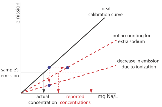
The solid black line in Figure 10.7.6 shows the ideal calibration curve, assuming we match the standard’s matrix to the sample’s matrix, and that we do so without adding any additional sodium. If we prepare the external standards without adding KCl, the emission for each standard decreases due to increased ionization. This is shown by the lower of the two dashed red lines. Preparing the standards by adding reagent grade KCl increases the concentration of sodium due to its contamination. Because we underestimate the actual concentration of sodium in the standards, the resulting calibration curve is shown by the other dashed red line. In both cases, the sample’s emission results in our overestimating the concentration of sodium in the sample.
4. One problem with analyzing salt samples is their tendency to clog the aspirator and burner assembly. What effect does this have on the analysis?
Clogging the aspirator and burner assembly decreases the rate of aspiration, which decreases the analyte’s concentration in the flame. The result is a decrease in the emission intensity and a negative determinate error.
To evaluate the method described in Representative Method 10.7.1, a series of standard additions is prepared using a 10.0077-g sample of a salt substitute. The results of a flame atomic emission analysis of the standards is shown here [Goodney, D. E. J. Chem. Educ. 1982, 59, 875–876].
| added Na (µg/mL) | Ie (arb. units) |
|---|---|
| 0.000 | 1.79 |
| 0.420 | 2.63 |
| 1.051 | 3.54 |
| 2.102 | 4.94 |
| 3.153 | 6.18 |
What is the concentration of sodium, in μg/g, in the salt substitute.
Solution
Linear regression of emission intensity versus the concentration of added Na gives the standard additions calibration curve shown below, which has the following calibration equation.

\[I_{e}=1.97+1.37 \times \frac{\mu \mathrm{g} \ \mathrm{Na}}{\mathrm{mL}} \nonumber\]
The concentration of sodium in the sample is the absolute value of the calibration curve’s x-intercept. Substituting zero for the emission intensity and solving for sodium’s concentration gives a result of 1.44 μgNa/mL. The concentration of sodium in the salt substitute is
\[\frac{\frac{1.44 \ \mu \mathrm{g} \ \mathrm{Na}}{\mathrm{mL}} \times \frac{50.00 \ \mathrm{mL}}{25.00 \ \mathrm{mL}} \times 250.0 \ \mathrm{mL}}{10.0077 \ \mathrm{g} \text { sample }}=71.9 \ \mu \mathrm{g} \ \mathrm{Na} / \mathrm{g}\nonumber\]
Evaluation of Atomic Emission Spectroscopy
Scale of Operation
The scale of operations for atomic emission is ideal for the direct analysis of trace and ultratrace analytes in macro and meso samples. With appropriate dilutions, atomic emission can be applied to major and minor analytes.
Accuracy
When spectral and chemical interferences are insignificant, atomic emission can achieve quantitative results with accuracies of 1–5%. For flame emission, accuracy frequently is limited by chemical interferences. Because the higher temperature of a plasma source gives rise to more emission lines, accuracy when using plasma emission often is limited by stray radiation from overlapping emission lines.
Precision
For samples and standards in which the analyte’s concentration exceeds the detection limit by at least a factor of 50, the relative standard deviation for both flame and plasma emission is about 1–5%. Perhaps the most important factor that affect precision is the stability of the flame’s or the plasma’s temperature. For example, in a 2500 K flame a temperature fluctuation of \(\pm 2.5\) K gives a relative standard deviation of 1% in emission intensity. Significant improvements in precision are realized when using internal standards.
Sensitivity
Sensitivity is influenced by the temperature of the excitation source and the composition of the sample matrix. Sensitivity is optimized by aspirating a standard solution of analyte and maximizing the emission by adjusting the flame’s composition and the height from which we monitor the emission. Chemical interferences, when present, decrease the sensitivity of the analysis. Because the sensitivity of plasma emission is less affected by the sample matrix, a calibration curve prepared using standards in a matrix of distilled water is possible even for samples that have more complex matrices.
Selectivity
The selectivity of atomic emission is similar to that of atomic absorption. Atomic emission has the further advantage of rapid sequential or simultaneous analysis of multiple analytes.
Time, Cost, and Equipment
Sample throughput with atomic emission is rapid when using an automated system that can analyze multiple analytes. For example, sampling rates of 3000 determinations per hour are possible using a multichannel ICP, and sampling rates of 300 determinations per hour when using a sequential ICP. Flame emission often is accomplished using an atomic absorption spectrometer, which typically costs between $10,000–$50,000. Sequential ICP’s range in price from $55,000–$150,000, while an ICP capable of simultaneous multielemental analysis costs between $80,000–$200,000. Combination ICP’s that are capable of both sequential and simultaneous analysis range in price from $150,000–$300,000. The cost of Ar, which is consumed in significant quantities, can not be overlooked when considering the expense of operating an ICP.