9.3: Complexation Titrations
- Page ID
- 165346

\( \newcommand{\vecs}[1]{\overset { \scriptstyle \rightharpoonup} {\mathbf{#1}} } \)
\( \newcommand{\vecd}[1]{\overset{-\!-\!\rightharpoonup}{\vphantom{a}\smash {#1}}} \)
\( \newcommand{\dsum}{\displaystyle\sum\limits} \)
\( \newcommand{\dint}{\displaystyle\int\limits} \)
\( \newcommand{\dlim}{\displaystyle\lim\limits} \)
\( \newcommand{\id}{\mathrm{id}}\) \( \newcommand{\Span}{\mathrm{span}}\)
( \newcommand{\kernel}{\mathrm{null}\,}\) \( \newcommand{\range}{\mathrm{range}\,}\)
\( \newcommand{\RealPart}{\mathrm{Re}}\) \( \newcommand{\ImaginaryPart}{\mathrm{Im}}\)
\( \newcommand{\Argument}{\mathrm{Arg}}\) \( \newcommand{\norm}[1]{\| #1 \|}\)
\( \newcommand{\inner}[2]{\langle #1, #2 \rangle}\)
\( \newcommand{\Span}{\mathrm{span}}\)
\( \newcommand{\id}{\mathrm{id}}\)
\( \newcommand{\Span}{\mathrm{span}}\)
\( \newcommand{\kernel}{\mathrm{null}\,}\)
\( \newcommand{\range}{\mathrm{range}\,}\)
\( \newcommand{\RealPart}{\mathrm{Re}}\)
\( \newcommand{\ImaginaryPart}{\mathrm{Im}}\)
\( \newcommand{\Argument}{\mathrm{Arg}}\)
\( \newcommand{\norm}[1]{\| #1 \|}\)
\( \newcommand{\inner}[2]{\langle #1, #2 \rangle}\)
\( \newcommand{\Span}{\mathrm{span}}\) \( \newcommand{\AA}{\unicode[.8,0]{x212B}}\)
\( \newcommand{\vectorA}[1]{\vec{#1}} % arrow\)
\( \newcommand{\vectorAt}[1]{\vec{\text{#1}}} % arrow\)
\( \newcommand{\vectorB}[1]{\overset { \scriptstyle \rightharpoonup} {\mathbf{#1}} } \)
\( \newcommand{\vectorC}[1]{\textbf{#1}} \)
\( \newcommand{\vectorD}[1]{\overrightarrow{#1}} \)
\( \newcommand{\vectorDt}[1]{\overrightarrow{\text{#1}}} \)
\( \newcommand{\vectE}[1]{\overset{-\!-\!\rightharpoonup}{\vphantom{a}\smash{\mathbf {#1}}}} \)
\( \newcommand{\vecs}[1]{\overset { \scriptstyle \rightharpoonup} {\mathbf{#1}} } \)
\(\newcommand{\longvect}{\overrightarrow}\)
\( \newcommand{\vecd}[1]{\overset{-\!-\!\rightharpoonup}{\vphantom{a}\smash {#1}}} \)
\(\newcommand{\avec}{\mathbf a}\) \(\newcommand{\bvec}{\mathbf b}\) \(\newcommand{\cvec}{\mathbf c}\) \(\newcommand{\dvec}{\mathbf d}\) \(\newcommand{\dtil}{\widetilde{\mathbf d}}\) \(\newcommand{\evec}{\mathbf e}\) \(\newcommand{\fvec}{\mathbf f}\) \(\newcommand{\nvec}{\mathbf n}\) \(\newcommand{\pvec}{\mathbf p}\) \(\newcommand{\qvec}{\mathbf q}\) \(\newcommand{\svec}{\mathbf s}\) \(\newcommand{\tvec}{\mathbf t}\) \(\newcommand{\uvec}{\mathbf u}\) \(\newcommand{\vvec}{\mathbf v}\) \(\newcommand{\wvec}{\mathbf w}\) \(\newcommand{\xvec}{\mathbf x}\) \(\newcommand{\yvec}{\mathbf y}\) \(\newcommand{\zvec}{\mathbf z}\) \(\newcommand{\rvec}{\mathbf r}\) \(\newcommand{\mvec}{\mathbf m}\) \(\newcommand{\zerovec}{\mathbf 0}\) \(\newcommand{\onevec}{\mathbf 1}\) \(\newcommand{\real}{\mathbb R}\) \(\newcommand{\twovec}[2]{\left[\begin{array}{r}#1 \\ #2 \end{array}\right]}\) \(\newcommand{\ctwovec}[2]{\left[\begin{array}{c}#1 \\ #2 \end{array}\right]}\) \(\newcommand{\threevec}[3]{\left[\begin{array}{r}#1 \\ #2 \\ #3 \end{array}\right]}\) \(\newcommand{\cthreevec}[3]{\left[\begin{array}{c}#1 \\ #2 \\ #3 \end{array}\right]}\) \(\newcommand{\fourvec}[4]{\left[\begin{array}{r}#1 \\ #2 \\ #3 \\ #4 \end{array}\right]}\) \(\newcommand{\cfourvec}[4]{\left[\begin{array}{c}#1 \\ #2 \\ #3 \\ #4 \end{array}\right]}\) \(\newcommand{\fivevec}[5]{\left[\begin{array}{r}#1 \\ #2 \\ #3 \\ #4 \\ #5 \\ \end{array}\right]}\) \(\newcommand{\cfivevec}[5]{\left[\begin{array}{c}#1 \\ #2 \\ #3 \\ #4 \\ #5 \\ \end{array}\right]}\) \(\newcommand{\mattwo}[4]{\left[\begin{array}{rr}#1 \amp #2 \\ #3 \amp #4 \\ \end{array}\right]}\) \(\newcommand{\laspan}[1]{\text{Span}\{#1\}}\) \(\newcommand{\bcal}{\cal B}\) \(\newcommand{\ccal}{\cal C}\) \(\newcommand{\scal}{\cal S}\) \(\newcommand{\wcal}{\cal W}\) \(\newcommand{\ecal}{\cal E}\) \(\newcommand{\coords}[2]{\left\{#1\right\}_{#2}}\) \(\newcommand{\gray}[1]{\color{gray}{#1}}\) \(\newcommand{\lgray}[1]{\color{lightgray}{#1}}\) \(\newcommand{\rank}{\operatorname{rank}}\) \(\newcommand{\row}{\text{Row}}\) \(\newcommand{\col}{\text{Col}}\) \(\renewcommand{\row}{\text{Row}}\) \(\newcommand{\nul}{\text{Nul}}\) \(\newcommand{\var}{\text{Var}}\) \(\newcommand{\corr}{\text{corr}}\) \(\newcommand{\len}[1]{\left|#1\right|}\) \(\newcommand{\bbar}{\overline{\bvec}}\) \(\newcommand{\bhat}{\widehat{\bvec}}\) \(\newcommand{\bperp}{\bvec^\perp}\) \(\newcommand{\xhat}{\widehat{\xvec}}\) \(\newcommand{\vhat}{\widehat{\vvec}}\) \(\newcommand{\uhat}{\widehat{\uvec}}\) \(\newcommand{\what}{\widehat{\wvec}}\) \(\newcommand{\Sighat}{\widehat{\Sigma}}\) \(\newcommand{\lt}{<}\) \(\newcommand{\gt}{>}\) \(\newcommand{\amp}{&}\) \(\definecolor{fillinmathshade}{gray}{0.9}\)The earliest examples of metal–ligand complexation titrations are Liebig’s determinations, in the 1850s, of cyanide and chloride using, respectively, Ag+ and Hg2+ as the titrant. Practical analytical applications of complexation titrimetry were slow to develop because many metals and ligands form a series of metal–ligand complexes. Liebig’s titration of CN– with Ag+ was successful because they form a single, stable complex of \(\text{Ag(CN)}_2^-\), which results in a single, easily identified end point. Other metal–ligand complexes, such as \(\text{CdI}_4^{2-}\), are not analytically useful because they form a series of metal–ligand complexes (CdI+, CdI2(aq), \(\text{CdI}_3^-\) and \(\text{CdI}_4^{2-}\)) that produce a sequence of poorly defined end points.
Recall that an acid–base titration curve for a diprotic weak acid has a single end point if its two Ka values are not sufficiently different. See Figure 9.2.6 for an example.
In 1945, Schwarzenbach introduced aminocarboxylic acids as multidentate ligands. The most widely used of these new ligands—ethylenediaminetetraacetic acid, or EDTA—forms a strong 1:1 complex with many metal ions. The availability of a ligand that gives a single, easily identified end point made complexation titrimetry a practical analytical method.
Chemistry and Properties of EDTA
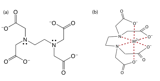
Ethylenediaminetetraacetic acid, or EDTA, is an aminocarboxylic acid. EDTA, the structure of which is shown in Figure 9.3.1 a in its fully deprotonated form, is a Lewis acid with six binding sites—the four negatively charged carboxylate groups and the two tertiary amino groups—that can donate up to six pairs of electrons to a metal ion. The resulting metal–ligand complex, in which EDTA forms a cage-like structure around the metal ion (Figure 9.3.1 b), is very stable. The actual number of coordination sites depends on the size of the metal ion, however, all metal–EDTA complexes have a 1:1 stoichiometry.
Metal–EDTA Formation Constants
To illustrate the formation of a metal–EDTA complex, let’s consider the reaction between Cd2+ and EDTA
\[\mathrm{Cd}^{2+}(a q)+\mathrm{Y}^{4-}(a q)\rightleftharpoons\mathrm{Cd} \mathrm{Y}^{2-}(a q) \label{9.1}\]
where Y4– is a shorthand notation for the fully deprotonated form of EDTA shown in Figure 9.3.1 a. Because the reaction’s formation constant
\[K_{f}=\frac{\left[\mathrm{CdY}^{2-}\right]}{\left[\mathrm{Cd}^{2+}\right]\left[\mathrm{Y}^{4-}\right]}=2.9 \times 10^{16} \label{9.2}\]
is large, its equilibrium position lies far to the right. Formation constants for other metal–EDTA complexes are found in Appendix 12.
EDTA is a Weak Acid
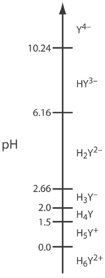
In addition to its properties as a ligand, EDTA is also a weak acid. The fully protonated form of EDTA, H6Y2+, is a hexaprotic weak acid with successive pKa values of
\[\mathrm{p} K_\text{a1}=0.0 \quad \mathrm{p} K_\text{a2}=1.5 \quad \mathrm{p} K_\text{a3}=2.0 \nonumber\]
\[\mathrm{p} K_\text{a4}=2.66 \quad \mathrm{p} K_\text{a5}=6.16 \quad \mathrm{p} K_\text{a6}=10.24 \nonumber\]
The first four values are for the carboxylic acid protons and the last two values are for the ammonium protons. Figure 9.3.2 shows a ladder diagram for EDTA. The specific form of EDTA in reaction \ref{9.1} is the predominate species only when the pH is more basic than 10.24.
Conditional Metal–Ligand Formation Constants
The formation constant for CdY2– in Equation \ref{9.2} assumes that EDTA is present as Y4–. Because EDTA has many forms, when we prepare a solution of EDTA we know it total concentration, CEDTA, not the concentration of a specific form, such as Y4–. To use Equation \ref{9.2}, we need to rewrite it in terms of CEDTA.
At any pH a mass balance on EDTA requires that its total concentration equal the combined concentrations of each of its forms.
\[C_{\mathrm{EDTA}}=\left[\mathrm{H}_{6} \mathrm{Y}^{2+}\right]+\left[\mathrm{H}_{5} \mathrm{Y}^{+}\right]+\left[\mathrm{H}_{4} \mathrm{Y}\right]+\left[\mathrm{H}_{3} \mathrm{Y}^-\right]+\left[\mathrm{H}_{2} \mathrm{Y}^{2-}\right]+\left[\mathrm{HY}^{3-}\right]+\left[\mathrm{Y}^{4-}\right] \nonumber\]
To correct the formation constant for EDTA’s acid–base properties we need to calculate the fraction, \(\alpha_{\text{Y}^{4-}}\), of EDTA that is present as Y4–.
\[\alpha_{\text{Y}^{4-}}=\frac{\left[\text{Y}^{4-}\right]}{C_\text{EDTA}} \label{9.3}\]
Table 9.3.1 provides values of \(\alpha_{\text{Y}^{4-}}\) for selected pH levels. Solving Equation \ref{9.3} for [Y4–] and substituting into Equation \ref{9.2} for the CdY2– formation constant
\[K_{\mathrm{f}}=\frac{\left[\mathrm{CdY}^{2-}\right]}{\left[\mathrm{Cd}^{2+}\right] (\alpha_{\mathrm{Y}^{4-}}) C_{\mathrm{EDTA}}} \nonumber\]
and rearranging gives
\[K_{f}^{\prime}=K_{f} \times \alpha_{\text{Y}^{4-}}=\frac{\left[\mathrm{CdY}^{2-}\right]}{\left[\mathrm{Cd}^{2+}\right] C_{\mathrm{EDTA}}} \label{9.4}\]
where \(K_f^{\prime}\) is a pH-dependent conditional formation constant. As shown in Table 9.3.2 , the conditional formation constant for CdY2– becomes smaller and the complex becomes less stable at more acidic pHs.
EDTA Competes With Other Ligands
To maintain a constant pH during a complexation titration we usually add a buffering agent. If one of the buffer’s components is a ligand that binds with Cd2+, then EDTA must compete with the ligand for Cd2+. For example, an \(\text{NH}_4^+ / \text{NH}_3\) buffer includes NH3, which forms several stable Cd2+–NH3 complexes. Because EDTA forms a stronger complex with Cd2+ than does NH3, it displaces NH3; however, the stability of the Cd2+–EDTA complex decreases.
We can account for the effect of an auxiliary complexing agent, such as NH3, in the same way we accounted for the effect of pH. Before adding EDTA, the mass balance on Cd2+, CCd, is
\[C_{\mathrm{Cd}} = \left[\mathrm{Cd}^{2+}\right] + \left[\mathrm{Cd}\left(\mathrm{NH}_{3}\right)^{2+}\right] + \left[\mathrm{Cd}\left(\mathrm{NH}_{3}\right)_{2}^{2+}\right] + \left[\mathrm{Cd}\left(\mathrm{NH}_{3}\right)_{3}^{2+}\right] + \left[\mathrm{Cd}\left(\mathrm{NH}_{3}\right)_{4}^{2+}\right] \nonumber\]
and the fraction of uncomplexed Cd2+, \(\alpha_{Cd^{2+}}\), is
\[\alpha_{\mathrm{Cd}^{2+}}=\frac{\left[\mathrm{Cd}^{2+}\right]}{C_{\mathrm{Cd}}} \label{9.5}\]
The value of \(\alpha_{\mathrm{Cd}^{2+}}\) depends on the concentration of NH3. Contrast this with \(\alpha_{\text{Y}^{4-}}\), which depends on pH.
Solving Equation \ref{9.5} for [Cd2+] and substituting into Equation \ref{9.4} gives
\[K_{f}^{\prime}=K_{f} \times \alpha_{Y^{4-}} = \frac {[\text{CdY}^{2-}]} {\alpha_{\text{Cd}^{2+}} C_\text{Cd} C_\text{EDTA}} \nonumber\]
Because the concentration of NH3 in a buffer essentially is constant, we can rewrite this equation
\[K_{f}^{\prime \prime}=K_{f} \times \alpha_{\mathrm{Y}^{4-}} \times \alpha_{\mathrm{Cd}^{2+}}=\frac{\left[\mathrm{CdY}^{2-}\right]}{C_{\mathrm{Cd}} C_{\mathrm{EDTA}}} \label{9.6}\]
to give a conditional formation constant, \(K_f^{\prime \prime}\), that accounts for both pH and the auxiliary complexing agent’s concentration. Table 9.3.3 provides values of \(\alpha_{\text{M}^{2+}}\) for several metal ion when NH3 is the complexing agent.
Complexometric EDTA Titration Curves
Now that we know something about EDTA’s chemical properties, we are ready to evaluate its usefulness as a titrant. To do so we need to know the shape of a complexometric titration curve. In chapter 9.2 we learned that an acid–base titration curve shows how the titrand’s pH changes as we add titrant. The analogous result for a complexation titration shows the change in pM, where M is the metal ion’s concentration, as a function of the volume of EDTA. In this section we will learn how to calculate a titration curve using the equilibrium calculations from Chapter 6. We also will learn how to sketch a good approximation of any complexation titration curve using a limited number of simple calculations.
pM = –log[M2+]
Calculating the Titration Curve
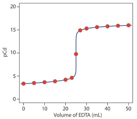
Let’s calculate the titration curve for 50.0 mL of \(5.00 \times 10^{-3}\) M Cd2+ using a titrant of 0.0100 M EDTA. Furthermore, let’s assume the titrand is buffered to a pH of 10 using a buffer that is 0.0100 M in NH3.
Because the pH is 10, some of the EDTA is present in forms other than Y4–. In addition, EDTA will compete with NH3 for the Cd2+. To evaluate the titration curve, therefore, we first need to calculate the conditional formation constant for CdY2–. From Table 9.3.1 and Table 9.3.3 we find that \(\alpha_{\text{Y}^{4-}}\) is 0.367 at a pH of 10, and that \(\alpha_{\text{Cd}^{2+}}\) is 0.0881 when the concentration of NH3 is 0.0100 M. Using these values, the conditional formation constant is
\[K_{f}^{\prime \prime}=K_{f} \times \alpha_{\text{Y}^{4-}} \times \alpha_{\text{Cd}^{2+}}=\left(2.9 \times 10^{16}\right)(0.367)(0.0881)=9.4 \times 10^{14} \nonumber\]
Because \(K_f^{\prime \prime}\) is so large, we can treat the titration reaction
\[\mathrm{Cd}^{2+}(a q)+\mathrm{Y}^{4-}(a q) \longrightarrow \mathrm{CdY}^{2-}(a q) \nonumber\]
as if it proceeds to completion.
The next task is to determine the volume of EDTA needed to reach the equivalence point. At the equivalence point we know that the moles of EDTA added must equal the moles of Cd2+ in our sample; thus
\[\operatorname{mol} \mathrm{EDTA}=M_{\mathrm{EDTA}} \times V_{\mathrm{EDTA}}=M_{\mathrm{Cd}} \times V_{\mathrm{Cd}}=\mathrm{mol} \ \mathrm{Cd}^{2+} \nonumber\]
Substituting in known values, we find that it requires
\[V_{eq}=V_{\mathrm{EDTA}}=\frac{M_{\mathrm{Cd}} V_{\mathrm{Cd}}}{M_{\mathrm{EDTA}}}=\frac{\left(5.00 \times 10^{-3} \ \mathrm{M}\right)(50.0 \ \mathrm{mL})}{0.0100 \ \mathrm{M}}=25.0 \ \mathrm{mL} \nonumber\]
of EDTA to reach the equivalence point.
Before the equivalence point, Cd2+ is present in excess and pCd is determined by the concentration of unreacted Cd2+. Because not all unreacted Cd2+ is free—some is complexed with NH3—we must account for the presence of NH3. For example, after adding 5.0 mL of EDTA, the total concentration of Cd2+ is
\[C_{\mathrm{Cd}} = \frac {(\text{mol Cd}^{2+})_\text{initial} - (\text{mol EDTA})_\text{added}} {\text{total volume}} = \frac {M_\text{Cd}V_\text{Cd} - M_\text{EDTA}V_\text{EDTA}} {V_\text{Cd} + V_\text{EDTA}} \nonumber\]
\[C_{\mathrm{Cd}}=\frac{\left(5.00 \times 10^{-3} \ \mathrm{M}\right)(50.0 \ \mathrm{mL})-(0.0100 \ \mathrm{M})(5.0 \ \mathrm{mL})}{50.0 \ \mathrm{mL}+5.0 \ \mathrm{mL}} \nonumber\]
\[C_{\mathrm{Cd}}=3.64 \times 10^{-3} \ \mathrm{M} \nonumber\]
To calculate the concentration of free Cd2+ we use Equation \ref{9.5}
\[\left[\mathrm{Cd}^{2+}\right]=\alpha_{\mathrm{Cd}^{2+}} \times C_{\mathrm{Cd}}=(0.0881)\left(3.64 \times 10^{-3} \ \mathrm{M}\right)=3.21 \times 10^{-4} \ \mathrm{M} \nonumber\]
which gives a pCd of
\[\mathrm{pCd}=-\log \left[\mathrm{Cd}^{2+}\right]=-\log \left(3.21 \times 10^{-4}\right)=3.49 \nonumber\]
At the equivalence point all Cd2+ initially in the titrand is now present as CdY2–. The concentration of Cd2+, therefore, is determined by the dissociation of the CdY2– complex. First, we calculate the concentration of CdY2–.
\[\left[\mathrm{CdY}^{2-}\right]=\frac{\left(\mathrm{mol} \ \mathrm{Cd}^{2+}\right)_{\mathrm{initial}}}{\text { total volume }} = \frac {M_\text{Cd}V_\text{Cd}} {V_\text{Cd} + V_\text{EDTA}} \nonumber\]
\[\left[\mathrm{CdY}^{2-}\right]=\frac{\left(5.00 \times 10^{-3} \ \mathrm{M}\right)(50.0 \ \mathrm{mL})}{50.0 \ \mathrm{mL}+25.0 \ \mathrm{mL}}=3.33 \times 10^{-3} \ \mathrm{M} \nonumber\]
Next, we solve for the concentration of Cd2+ in equilibrium with CdY2–.
\[K_{\mathrm{f}}^{\prime \prime}=\frac{\left[\mathrm{CdY}^{2-}\right]}{C_{\mathrm{Cd}} C_{\mathrm{EDTA}}}=\frac{3.33 \times 10^{-3}-x}{(x)(x)}=9.5 \times 10^{14} \nonumber\]
\[x=C_{\mathrm{Cd}}=1.87 \times 10^{-9} \ \mathrm{M} \nonumber\]
In calculating that [CdY2–] at the equivalence point is \(3.33 \times 10^{-3}\) M, we assumed the reaction between Cd2+ and EDTA went to completion. Here we let the system relax back to equilibrium, increasing CCd and CEDTA from 0 to x, and decreasing the concentration of CdY2– by x.
Once again, to find the concentration of uncomplexed Cd we must account for the presence of NH3; thus
\[\left[\mathrm{Cd}^{2+}\right]=\alpha_{\mathrm{Cd}^{2+}} \times C_{\mathrm{Cd}}=(0.0881)\left(1.87 \times 10^{-9} \ \mathrm{M}\right)=1.64 \times 10^{-10} \ \mathrm{M} \nonumber\]
and pCd is 9.78 at the equivalence point.
After the equivalence point, EDTA is in excess and the concentration of Cd2+ is determined by the dissociation of the CdY2– complex. First, we calculate the concentrations of CdY2– and of unreacted EDTA. For example, after adding 30.0 mL of EDTA the concentration of CdY2– is
\[\left[\mathrm{CdY}^{2-}\right]=\frac{\left(\mathrm{mol} \mathrm{Cd}^{2+}\right)_{\mathrm{initial}}}{\text { total volume }} = \frac{M_{\mathrm{Cd}} V_{\mathrm{Cd}}}{V_{\mathrm{Cd}}+V_{\mathrm{EDTA}}} \nonumber\]
\[\left[\mathrm{CdY}^{2-}\right]=\frac{\left(5.00 \times 10^{-3} \ \mathrm{M}\right)(50.0 \ \mathrm{mL})}{50.0 \ \mathrm{mL}+30.0 \ \mathrm{mL}}=3.12 \times 10^{-3} \ \mathrm{M} \nonumber\]
and the concentration of EDTA is
\[C_{\mathrm{EDTA}} = \frac {(\text{mol EDTA})_\text{added} - (\text{mol Cd}^{2+})_\text{initial}} {\text{total volume}} = \frac{M_{\mathrm{EDTA}} V_{\mathrm{EDTA}}-M_{\mathrm{Cd}} V_{\mathrm{Cd}}}{V_{\mathrm{Cd}}+V_{\mathrm{EDTA}}} \nonumber\]
\[C_{\text{EDTA}} = \frac {(0.0100 \text{ M})(30.0 \text{ mL}) - (5.00 \times 10^{-3} \text{ M})(50.0 \text{ mL})} {50.0 \text{ mL} + 30.0 \text{ mL}} \nonumber\]
\[C_{\mathrm{EDTA}}=6.25 \times 10^{-4} \ \mathrm{M} \nonumber\]
Substituting into Equation \ref{9.6} and solving for [Cd2+] gives
\[\frac{\left[\mathrm{CdY}^{2-}\right]}{C_{\mathrm{Cd}} C_{\mathrm{EDTA}}} = \frac{3.12 \times 10^{-3} \ \mathrm{M}}{C_{\mathrm{Cd}}\left(6.25 \times 10^{-4} \ \mathrm{M}\right)} = 9.5 \times 10^{14} \nonumber\]
\[C_{\text{Cd}} = 5.27 \times 10^{-15} \text{ M} \nonumber\]
\[ \left[ \text{Cd}^{2+} \right] = \alpha_{\text{Cd}^{2+}} \times C_{\text{Cd}} = (0.0881)(5.27 \times 10^{-15} \text{ M}) = 4.64 \times 10^{-16} \text{ M} \nonumber\]
a pCd of 15.33. Table 9.3.4 and Figure 9.3.3 show additional results for this titration.
After the equilibrium point we know the equilibrium concentrations of CdY2- and of EDTA in all its forms, CEDTA. We can solve for CCd using \(K_f^{\prime \prime}\) and then calculate [Cd2+] using \(\alpha_{\text{Cd}^{2+}}\). Because we used the same conditional formation constant, \(K_f^{\prime \prime}\), for other calculations in this section, this is the approach used here as well. There is a second method for calculating [Cd2+] after the equivalence point. Because the calculation uses only [CdY2-] and CEDTA, we can use \(K_f^{\prime}\) instead of \(K_f^{\prime \prime}\); thus
\[\frac{\left[\mathrm{CdY}^{2-}\right]}{\left[\mathrm{Cd}^{2+}\right] C_{\mathrm{EDTA}}}=\alpha_{\mathrm{Y}^{4-}} \times K_{\mathrm{f}} \nonumber\]
\[\frac{3.13 \times 10^{-3} \ \mathrm{M}}{\left[\mathrm{Cd}^{2+}\right]\left(6.25 \times 10^{-4}\right)}=(0.367)\left(2.9 \times 10^{16}\right) \nonumber\]
Solving gives [Cd2+] = \(4.71 \times 10^{-16}\) M and a pCd of 15.33. We will use this approach when we learn how to sketch a complexometric titration curve.
Calculate titration curves for the titration of 50.0 mL of \(5.00 \times 10^{-3}\) M Cd2+ with 0.0100 M EDTA (a) at a pH of 10 and (b) at a pH of 7. Neither titration includes an auxiliary complexing agent. Compare your results with Figure 9.3.3 and comment on the effect of pH on the titration of Cd2+ with EDTA.
- Answer
-
Let’s begin with the calculations at a pH of 10 where some of the EDTA is present in forms other than Y4–. To evaluate the titration curve, therefore, we need the conditional formation constant for CdY2–, which, from Table 9.3.2 is \(K_f^{\prime} = 1.1 \times 10^{16}\). Note that the conditional formation constant is larger in the absence of an auxiliary complexing agent.
The titration’s equivalence point requires
\[V_{e q}=V_{\mathrm{EDTA}}=\frac{M_{\mathrm{Cd}} V_{\mathrm{Cd}}}{M_{\mathrm{EDTA}}}=\frac{\left(5.00 \times 10^{-3} \ \mathrm{M}\right)(50.0 \ \mathrm{mL})}{(0.0100 \ \mathrm{M})}=25.0 \ \mathrm{mL} \nonumber\]
of EDTA.
Before the equivalence point, Cd2+ is present in excess and pCd is determined by the concentration of unreacted Cd2+. For example, after adding 5.00 mL of EDTA, the total concentration of Cd2+ is
\[\left[\mathrm{Cd}^{2+}\right]=\frac{\left(5.00 \times 10^{-3} \ \mathrm{M}\right)(50.0 \ \mathrm{mL})-(0.0100 \ \mathrm{M})(5.00 \ \mathrm{mL})}{50.0 \ \mathrm{mL}+5.00 \ \mathrm{mL}} \nonumber\]
which gives [Cd2+] as \(3.64 \times 10^{-3}\) and pCd as 2.43.
At the equivalence point all Cd2+ initially in the titrand is now present as CdY2–. The concentration of Cd2+, therefore, is determined by the dissociation of the CdY2– complex. First, we calculate the concentration of CdY2–.
\[\left[\mathrm{CdY}^{2-}\right]=\frac{\left(5.00 \times 10^{-3} \ \mathrm{M}\right)(50.0 \ \mathrm{mL})}{50.0 \ \mathrm{mL}+25.00 \ \mathrm{mL}}=3.33 \times 10^{-3} \ \mathrm{M} \nonumber\]
Next, we solve for the concentration of Cd2+ in equilibrium with CdY2–.
\[K_{f}^{\prime}=\frac{\left[\mathrm{CdY}^{2-}\right]}{\left[\mathrm{Cd}^{2+}\right] C_{\mathrm{EDTA}}}=\frac{3.33 \times 10^{-3}-x}{(x)(x)}=1.1 \times 10^{16} \nonumber\]
Solving gives [Cd2+] as \(5.50 \times 10^{-10}\) M or a pCd of 9.26 at the equivalence point.
After the equivalence point, EDTA is in excess and the concentration of Cd2+ is determined by the dissociation of the CdY2– complex. First, we calculate the concentrations of CdY2– and of unreacted EDTA. For example, after adding 30.0 mL of EDTA
\[\left[\mathrm{CdY}^{2-}\right]=\frac{\left(5.00 \times 10^{-3} \ \mathrm{M}\right)(50.0 \ \mathrm{mL})}{50.0 \ \mathrm{mL}+30.00 \ \mathrm{mL}}=3.12 \times 10^{-3} \ \mathrm{M} \nonumber\]
\[C_{\mathrm{EDTA}}=\frac{(0.0100 \ \mathrm{M})(30.00 \ \mathrm{mL})-\left(5.00 \times 10^{-3} \ \mathrm{M}\right)(50.0 \ \mathrm{mL})}{50.0 \ \mathrm{mL}+30.00 \ \mathrm{mL}} \nonumber\]
\[C_{\mathrm{EDTA}}=6.25 \times 10^{-4} \ \mathrm{M} \nonumber\]
Substituting into the equation for the conditional formation constant
\[K_{f}^{\prime}=\frac{\left[\mathrm{CdY}^{2-}\right]}{\left[\mathrm{Cd}^{2+}\right] C_{\mathrm{EDTA}}}=\frac{3.12 \times 10^{-3} \ \mathrm{M}}{(\mathrm{x})\left(6.25 \times 10^{-4} \ \mathrm{M}\right)}=1.1 \times 10^{16} \nonumber\]
and solving for [Cd2+] gives \(4.54 \times 10^{-16}\) M or a pCd of 15.34.
The calculations at a pH of 7 are identical, except the conditional formation constant for CdY2– is \(1.5 \times 10^{13}\) instead of \(1.1 \times 10^{16}\). The following table summarizes results for these two titrations as well as the results from Table 9.3.4 for the titration of Cd2+ at a pH of 10 in the presence of 0.0100 M NH3 as an auxiliary complexing agent.
Volume of EDTA (mL)
pCd at pH 10
pCd at pH 10 w/ 0.0100 M NH3
pCd at pH 7
0 2.30
3.36
2.30
5.00
2.43
3.49
2.43
10.0 2.60
3.66
2.60
15.0 2.81
3.87
2.81
20.0 3.15
4.20
3.15
23.0 3.56
4.62
3.56
25.0 9.26
9.77
7.83
27.0 14.94 14.95 12.08
30.0 15.34 15.33 12.48 35.0 15.61 15.61 12.78 40.0 15.76 15.76 12.95 45.0 15.86 15.86 13.08 50.0 15.94 15.94 13.18 Examining these results allows us to draw several conclusions. First, in the absence of an auxiliary complexing agent the titration curve before the equivalence point is independent of pH (compare columns 2 and 4). Second, for any pH, the titration curve after the equivalence point is the same regardless of whether an auxiliary complexing agent is present (compare columns 2 and 3). Third, the largest change in pH through the equivalence point occurs at higher pHs and in the absence of an auxiliary complexing agent. For example, from 23.0 mL to 27.0 mL of EDTA the change in pCd is 11.38 at a pH of 10, 10.33 at a pH of 10 in the presence of 0.0100 M NH3, and 8.52 at a pH of 7.
Sketching an EDTA Titration Curve
To evaluate the relationship between a titration’s equivalence point and its end point, we need to construct only a reasonable approximation of the exact titration curve. In this section we demonstrate a simple method for sketching a complexation titration curve. Our goal is to sketch the titration curve quickly, using as few calculations as possible. Let’s use the titration of 50.0 mL of \(5.00 \times 10^{-3}\) M Cd2+ with 0.0100 M EDTA in the presence of 0.0100 M NH3 to illustrate our approach. This is the same example we used in developing the calculations for a complexation titration curve. You can review the results of that calculation in Table 9.3.4 and Figure 9.3.3 .
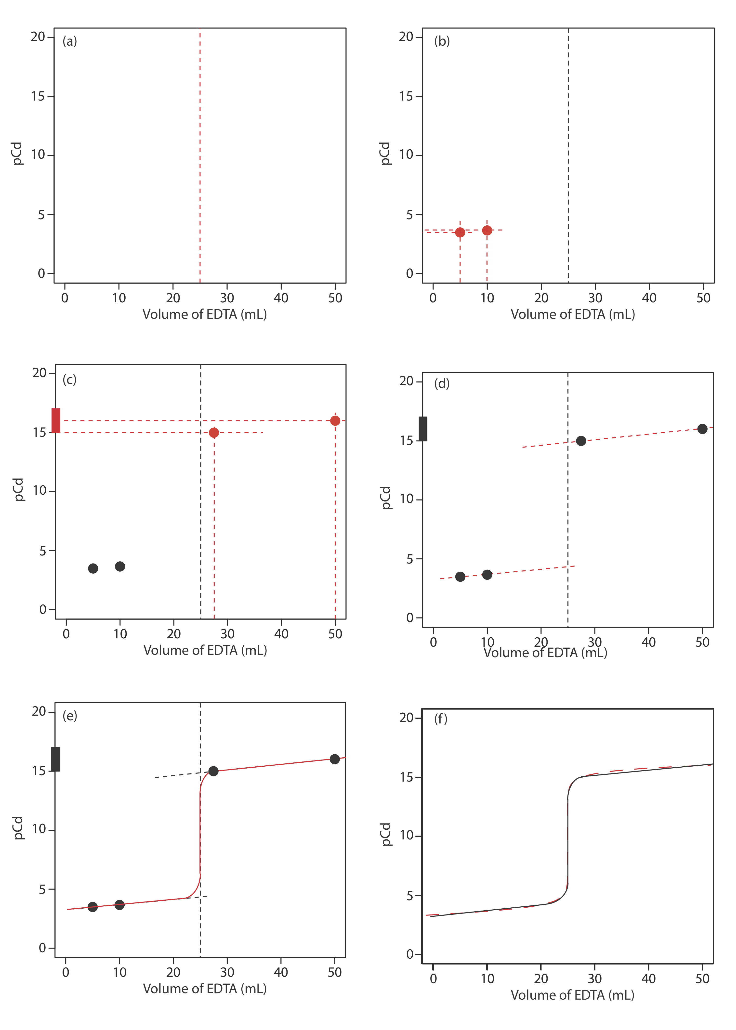
We begin by calculating the titration’s equivalence point volume, which, as we determined earlier, is 25.0 mL. Next, we draw our axes, placing pCd on the y-axis and the titrant’s volume on the x-axis. To indicate the equivalence point’s volume, we draw a vertical line that intersects the x-axis at 25.0 mL of EDTA. Figure 9.3.4 a shows the result of the first step in our sketch.
Before the equivalence point, Cd2+ is present in excess and pCd is determined by the concentration of unreacted Cd2+. Because not all unreacted Cd2+ is free—some is complexed with NH3—we must account for the presence of NH3. The calculations are straightforward, as we saw earlier. Figure 9.3.4 b shows the pCd after adding 5.00 mL and 10.0 mL of EDTA.
The third step in sketching our titration curve is to add two points after the equivalence point. Here the concentration of Cd2+ is controlled by the dissociation of the Cd2+–EDTA complex. Beginning with the conditional formation constant
\[K_{f}^{\prime}=\frac{\left[\mathrm{CdY}^{2-}\right]}{\left[\mathrm{Cd}^{2+}\right] C_{\mathrm{EDTA}}} = \alpha_{\text{Y}^{4-}} \times K_{f}=(0.367)\left(2.9 \times 10^{16}\right)=1.1 \times 10^{16} \nonumber\]
we take the log of each side and rearrange, arriving at
\[\begin{array}{c}{\log K_{f}^{\prime}=-\log \left[\mathrm{Cd}^{2+}\right]+\log \frac{\left[\mathrm{CdY}^{2-}\right]}{C_{\mathrm{EDTA}}}} \\ {\mathrm{pCd}=\log K_{f}^{\prime}+\log \frac{C_{\mathrm{EDTA}}}{\left[\mathrm{CdY}^{2-}]\right.}}\end{array} \nonumber\]
Recall that we can use either of our two possible conditional formation constants, \(K_f^{\prime}\) or \(K_f^{\prime \prime}\), to determine the composition of the system at equilibrium.
Note that after the equivalence point, the titrand is a metal–ligand complexation buffer, with pCd determined by CEDTA and [CdY2–]. The buffer is at its lower limit of \(\text{pCd} = \log{K_f^{\prime}} - 1\) when
\[\frac{C_{\mathrm{EDTA}}}{\left[\mathrm{CdY}^{2-}\right]} = \frac {(\text{mole EDTA})_\text{added} - (\text{mol Cd}^{2+})_\text{initial}} {(\text{mol Cd}^{2+})_\text{initial}} = \frac {1} {10} \nonumber\]
Making appropriate substitutions and solving, we find that
\[\frac{M_{\mathrm{EDTA}} V_{\mathrm{EDTA}}-M_{\mathrm{Cd}} V_{\mathrm{Cd}}}{M_{\mathrm{Cd}} V_{\mathrm{Cd}}}=\frac{1}{10} \nonumber\]
\[M_{\mathrm{EDTA}} V_{\mathrm{EDTA}}-M_{\mathrm{Cd}} V_{\mathrm{Cd}}=0.1 \times M_{\mathrm{Cd}} V_{\mathrm{Cd}} \nonumber\]
\[V_{\mathrm{EDTA}}=\frac{1.1 \times M_{\mathrm{Cd}} V_{\mathrm{Cd}}}{M_{\mathrm{EDTA}}}=1.1 \times V_{e q} \nonumber\]
Thus, when the titration reaches 110% of the equivalence point volume, pCd is \(\log{K_f^{\prime}} - 1\). A similar calculation should convince you that pCd is \(\log{K_f^{\prime}} + 1\) when the volume of EDTA is \(2 \times V_\text{eq}\).
Figure 9.3.4 c shows the third step in our sketch. First, we add a ladder diagram for the CdY2– complex, including its buffer range, using its \(\log{K_f^{\prime}}\) value of 16.04. Next, we add two points, one for pCd at 110% of Veq (a pCd of 15.04 at 27.5 mL) and one for pCd at 200% of Veq (a pCd of 16.04 at 50.0 mL).
Next, we draw a straight line through each pair of points, extending each line through the vertical line that indicates the equivalence point’s volume (Figure 9.3.4 d). Finally, we complete our sketch by drawing a smooth curve that connects the three straight-line segments (Figure 9.3.4 e). A comparison of our sketch to the exact titration curve (Figure 9.3.4 f) shows that they are in close agreement.
Our treatment here is general and applies to any complexation titration using EDTA as a titrant.
Sketch titration curves for the titration of 50.0 mL of \(5.00 \times 10^{-3}\) M Cd2+ with 0.0100 M EDTA (a) at a pH of 10 and (b) at a pH of 7. Compare your sketches to the calculated titration curves from Exercise 9.3.1 .
- Answer
-
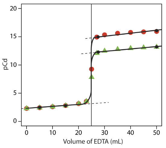
The figure below shows a sketch of the titration curves. The two black points before the equivalence point (VEDTA = 5 mL, pCd= 2.43 and VEDTA = 15 mL, pCd= 2.81) are the same for both pHs and taken from the results of Exercise 9.3.1 . The two black points after the equivalence point for a pH of 7 (VEDTA = 27.5 mL, pCd= 12.2 and VEDTA = 50 mL, pCd= 13.2) are plotted using the \(\log{K_f^{\prime}}\) of 13.2 for CdY2-. The two points after the equivalence point for a pH of 10 (VEDTA = 27.5 mL, pCd= 15.0 andVEDTA = 50 mL, pCd= 16.0) are plotted using the \(\log{K_f^{\prime}}\) of 16.0 for CdY2-. The points in red are the calculations from Exercise 9.3.1 for a pH of 10, and the points in green are the calculations from Exercise 9.3.1 for a pH of 7.
Selecting and Evaluating the Endpoint
The equivalence point of a complexation titration occurs when we react stoichiometrically equivalent amounts of the titrand and titrant. As is the case for an acid–base titration, we estimate the equivalence point for a complexation titration using an experimental end point. A variety of methods are available for locating the end point, including indicators and sensors that respond to a change in the solution conditions.
Finding the End Point with an Indicator
Most indicators for complexation titrations are organic dyes—known as metallochromic indicators—that form stable complexes with metal ions. The indicator, Inm–, is added to the titrand’s solution where it forms a stable complex with the metal ion, MInn–. As we add EDTA it reacts first with free metal ions, and then displaces the indicator from MInn–.
\[\text{MIn}^{n-}(aq) + \text{Y}^{4-}(aq) \rightarrow \text{MY}^{2-}(aq) + \text{In}^{m-}(aq) \nonumber\]
If MInn– and Inm– have different colors, then the change in color signals the end point.
The accuracy of an indicator’s end point depends on the strength of the metal–indicator complex relative to the strength of the metal–EDTA complex. If the metal–indicator complex is too strong, the change in color occurs after the equivalence point. If the metal–indicator complex is too weak, however, the end point occurs before we reach the equivalence point.
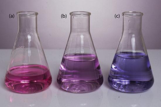
Most metallochromic indicators also are weak acids. One consequence of this is that the conditional formation constant for the metal–indicator complex depends on the titrand’s pH. This provides some control over an indicator’s titration error because we can adjust the strength of a metal–indicator complex by adjusted the pH at which we carry out the titration. Unfortunately, because the indicator is a weak acid, the color of the uncomplexed indicator also may change with pH. Figure 9.3.5 , for example, shows the color of the indicator calmagite as a function of pH and pMg, where H2In–, HIn2–, and In3– are different forms of the uncomplexed indicator, and MgIn– is the Mg2+–calmagite complex. Because the color of calmagite’s metal–indicator complex is red, its use as a metallochromic indicator has a practical pH range of approximately 8.5–11 where the uncomplexed indicator, HIn2–, has a blue color.
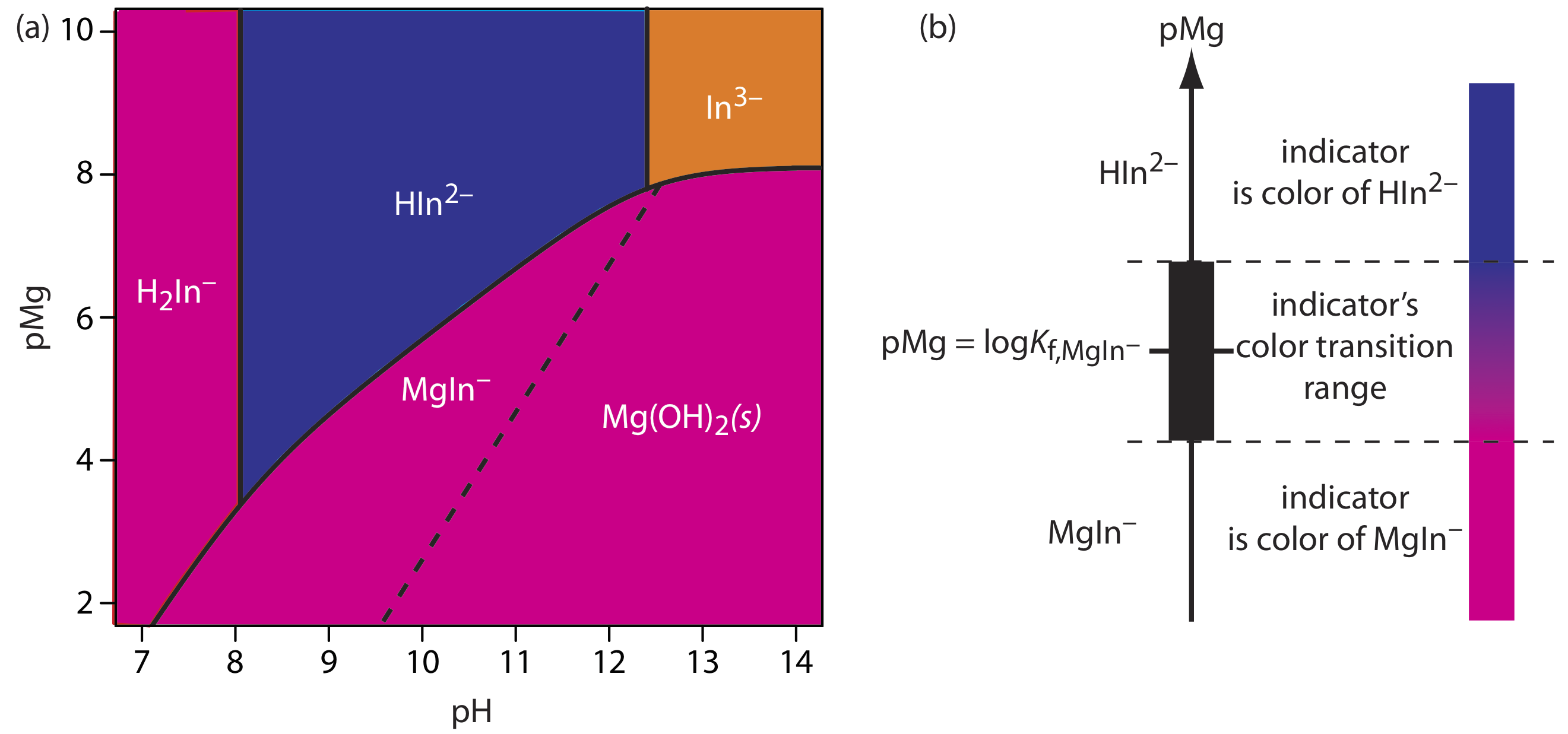
Table 9.3.5 provides examples of metallochromic indicators and the metal ions and pH conditions for which they are useful. Even if a suitable indicator does not exist, it often is possible to complete an EDTA titration by introducing a small amount of a secondary metal–EDTA complex if the secondary metal ion forms a stronger complex with the indicator and a weaker complex with EDTA than the analyte. For example, calmagite has a poor end point when titrating Ca2+ with EDTA. Adding a small amount of Mg2+–EDTA to the titrand gives a sharper end point. Because Ca2+ forms a stronger complex with EDTA, it displaces Mg2+, which then forms the red-colored Mg2+–calmagite complex. At the titration’s end point, EDTA displaces Mg2+ from the Mg2+–calmagite complex, signaling the end point by the presence of the uncomplexed indicator’s blue form.
Finding the End Point By Monitoring Absorbance
An important limitation when using a metallochromic indicator is that we must be able to see the indicator’s change in color at the end point. This may be difficult if the solution is already colored. For example, when titrating Cu2+ with EDTA, ammonia is used to adjust the titrand’s pH. The intensely colored \(\text{Cu(NH}_3)_2^{4+}\) complex obscures the indicator’s color, making an accurate determination of the end point difficult. Other absorbing species present within the sample matrix may also interfere. This often is a problem when analyzing clinical samples, such as blood, or environmental samples, such as natural waters.
If at least one species in a complexation titration absorbs electromagnet- ic radiation, then we can identify the end point by monitoring the titrand’s absorbance at a carefully selected wavelength. For example, we can identify the end point for a titration of Cu2+ with EDTA in the presence of NH3 by monitoring the titrand’s absorbance at a wavelength of 745 nm, where the \(\text{Cu(NH}_3)_2^{4+}\) complex absorbs strongly. At the beginning of the titration the absorbance is at a maximum. As we add EDTA, however, the reaction
\[\text{Cu(NH}_3)_4^{2+}(aq) + \text{Y}^{4-} \rightleftharpoons \text{CuY}^{2-}(aq) + 4\text{NH}_3(aq) \nonumber\]
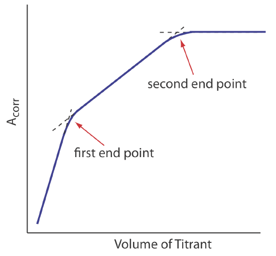
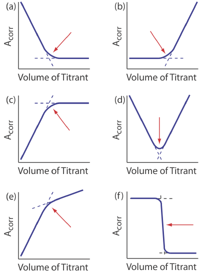
decreases the concentration of \(\text{Cu(NH}_3)_2^{4+}\) and decreases the absorbance until we reach the equivalence point. After the equivalence point the absorbance essentially remains unchanged. The resulting spectrophotometric titration curve is shown in Figure 9.3.6 a. Note that the titration curve’s y-axis is not the measured absorbance, Ameas, but a corrected absorbance, Acorr
\[A_\text{corr} = A_\text{meas} \times \frac {V_\text{EDTA} + V_\text{Cu}} {V_\text{Cu}} \nonumber\]
where VEDTA and VCu are, respectively, the volumes of EDTA and Cu. Correcting the absorbance for the titrand’s dilution ensures that the spectrophotometric titration curve consists of linear segments that we can extrapolate to find the end point. Other common spectrophotometric titration curves are shown in Figures 9.3.6 b-f.
Representative Method 9.3.1: Determination of Hardness of Water and Wastewater
The best way to appreciate the theoretical and the practical details discussed in this section is to carefully examine a typical complexation titrimetric method. Although each method is unique, the following description of the determination of the hardness of water provides an instructive example of a typical procedure. The description here is based on Method 2340C as published in Standard Methods for the Examination of Water and Wastewater, 20th Ed., American Public Health Association: Washington, D. C., 1998.
Description of the Method
The operational definition of water hardness is the total concentration of cations in a sample that can form an insoluble complex with soap. Although most divalent and trivalent metal ions contribute to hardness, the two most important metal ions are Ca2+ and Mg2+. Hardness is determined by titrating with EDTA at a buffered pH of 10. Calmagite is used as an indicator. Hardness is reported as mg CaCO3/L.
Procedure
Select a volume of sample that requires less than 15 mL of titrant to keep the analysis time under 5 minutes and, if necessary, dilute the sample to 50 mL with distilled water. Adjust the sample’s pH by adding 1–2 mL of a pH 10 buffer that contains a small amount of Mg2+–EDTA. Add 1–2 drops of indicator and titrate with a standard solution of EDTA until the red-to-blue end point is reached (Figure 9.3.7 ).
Questions
1. Why is the sample buffered to a pH of 10? What problems might you expect at a higher pH or a lower pH?
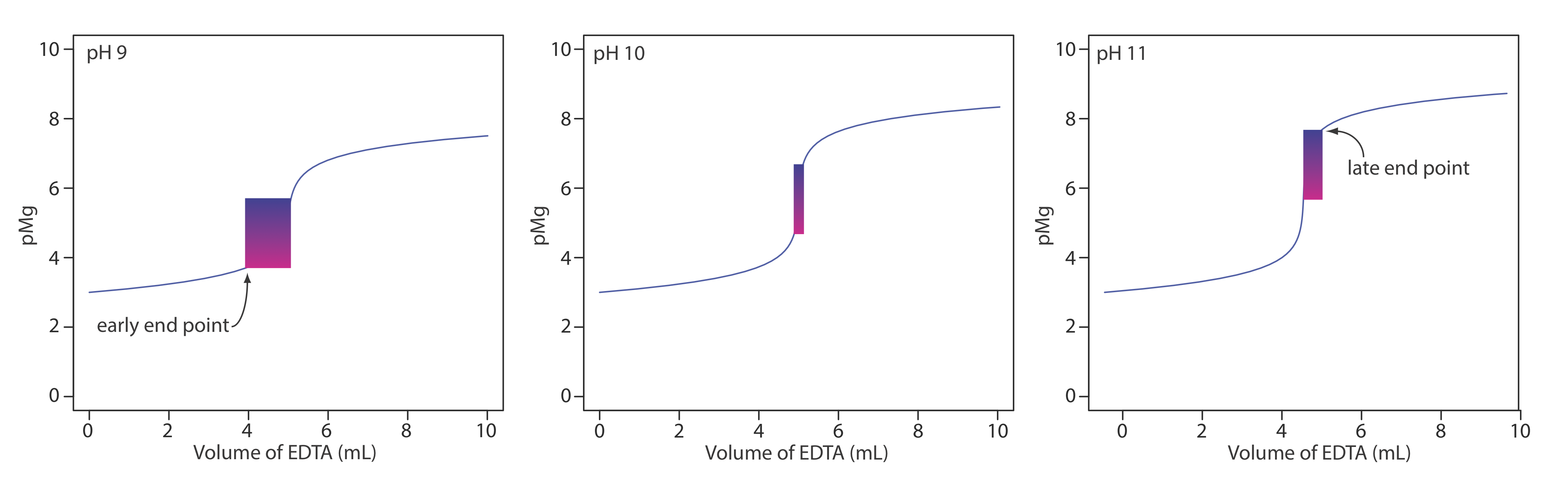
Of the two primary cations that contribute to hardness, Mg2+ forms the weaker complex with EDTA and is the last cation to react with the titrant. Calmagite is a useful indicator because it gives a distinct end point when titrating Mg2+ (see Table 9.3.5 ). Because of calmagite’s acid–base properties, the range of pMg values over which the indicator changes color depends on the titrand’s pH (Figure 9.3.5 ). Figure 9.3.8 shows the titration curve for a 50-mL solution of 10–3 M Mg2+ with 10–2 M EDTA at pHs of 9, 10, and 11. Superimposed on each titration curve is the range of conditions for which the average analyst will observe the end point. At a pH of 9 an early end point is possible, which results in a negative determinate error. A late end point and a positive determinate error are possible if the pH is 11.
2. Why is a small amount of the Mg2+–EDTA complex added to the buffer?
The titration’s end point is signaled by the indicator calmagite. The indicator’s end point with Mg2+ is distinct, but its change in color when titrating Ca2+ does not provide a good end point (see Table 9.3.5 ). If the sample does not contain any Mg2+ as a source of hardness, then the titration’s end point is poorly defined, which leads to an inaccurate and imprecise result. Adding a small amount of Mg2+–EDTA to the buffer ensures that the titrand includes at least some Mg2+. Because Ca2+ forms a stronger complex with EDTA, it displaces Mg2+ from the Mg2+–EDTA complex, freeing the Mg2+ to bind with the indicator. This displacement is stoichiometric, so the total concentration of hardness cations remains unchanged. The displacement by EDTA of Mg2+ from the Mg2+–indicator complex signals the titration’s end point.
3. Why does the procedure specify that the titration take no longer than 5 minutes?
A time limitation suggests there is a kinetically-controlled interference, possibly arising from a competing chemical reaction. In this case the interference is the possible precipitation of CaCO3 at a pH of 10.
Quantitative Applications
Although many quantitative applications of complexation titrimetry have been replaced by other analytical methods, a few important applications continue to find relevance. In the section we review the general application of complexation titrimetry with an emphasis on applications from the analysis of water and wastewater. First, however, we discuss the selection and standardization of complexation titrants.
Selection and Standardization of Titrants
EDTA is a versatile titrant that can be used to analyze virtually all metal ions. Although EDTA is the usual titrant when the titrand is a metal ion, it cannot be used to titrate anions, for which Ag+ or Hg2+ are suitable titrants.
Solutions of EDTA are prepared from its soluble disodium salt, Na2H2Y•2H2O, and standardized by titrating against a solution made from the primary standard CaCO3. Solutions of Ag+ and Hg2+ are prepared using AgNO3 and Hg(NO3)2, both of which are secondary standards. Standardization is accomplished by titrating against a solution prepared from primary standard grade NaCl.
Inorganic Analytes
Complexation titrimetry continues to be listed as a standard method for the determination of hardness, Ca2+, CN–, and Cl– in waters and wastewaters. The evaluation of hardness was described earlier in Representative Method 9.3.1. The determination of Ca2+ is complicated by the presence of Mg2+, which also reacts with EDTA. To prevent an interference the pH is adjusted to 12–13, which precipitates Mg2+ as Mg(OH)2. Titrating with EDTA using murexide or Eriochrome Blue Black R as the indicator gives the concentration of Ca2+.
Cyanide is determined at concentrations greater than 1 mg/L by making the sample alkaline with NaOH and titrating with a standard solution of AgNO3 to form the soluble \(\text{Ag(CN)}_2^-\) complex. The end point is determined using p-dimethylaminobenzalrhodamine as an indicator, with the solution turning from a yellow to a salmon color in the presence of excess Ag+.
Chloride is determined by titrating with Hg(NO3)2, forming HgCl2(aq). The sample is acidified to a pH of 2.3–3.8 and diphenylcarbazone, which forms a colored complex with excess Hg2+, serves as the indicator. The pH indicator xylene cyanol FF is added to ensure that the pH is within the desired range. The initial solution is a greenish blue, and the titration is carried out to a purple end point.
Quantitative Calculations
The quantitative relationship between the titrand and the titrant is determined by the titration reaction’s stoichiometry. For a titration using EDTA, the stoichiometry is always 1:1.
The concentration of a solution of EDTA is determined by standardizing against a solution of Ca2+ prepared using a primary standard of CaCO3. A 0.4071-g sample of CaCO3 is transferred to a 500-mL volumetric flask, dissolved using a minimum of 6 M HCl, and diluted to volume. After transferring a 50.00-mL portion of this solution to a 250-mL Erlenmeyer flask, the pH is adjusted by adding 5 mL of a pH 10 NH3–NH4Cl buffer that contains a small amount of Mg2+–EDTA. After adding calmagite as an indicator, the solution is titrated with the EDTA, requiring 42.63 mL to reach the end point. Report the molar concentration of EDTA in the titrant.
Solution
The primary standard of Ca2+ has a concentration of
\[\frac {0.4071 \text{ g CaCO}_3}{0.5000 \text{ L}} \times \frac {1 \text{ mol Ca}^{2+}}{100.09 \text{ g CaCO}_3} = 8.135 \times 10^{-3} \text{ M Ca}^{2+} \nonumber\]
The moles of Ca2+ in the titrand is
\[8.135 \times 10^{-3} \text{ M Ca}^{2+} \times 0.05000 \text{ L} = 4.068 \times 10^{-4} \text{ mol Ca}^{2+} \nonumber\]
which means that \(4.068 \times 10^{-4}\) moles of EDTA are used in the titration. The molarity of EDTA in the titrant is
\[\frac {4.068 \times 10^{-4} \text{ mol Ca}^{2+}}{0.04263 \text{ L}} = 9.543 \times 10^{-3} \text{ M EDTA} \nonumber\]
A 100.0-mL sample is analyzed for hardness using the procedure outlined in Representative Method 9.3.1, requiring 23.63 mL of 0.0109 M EDTA. Report the sample’s hardness as mg CaCO3/L.
- Answer
-
In an analysis for hardness we treat the sample as if Ca2+ is the only metal ion that reacts with EDTA. The grams of Ca2+ in the sample, therefore, are
\[(0.0109 \text{ M EDTA})(0.02363 \text{ L}) \times \frac {1 \text{ mol Ca}^{2+}}{\text{mol EDTA}} = 2.58 \times 10^{-4} \text{ mol Ca}^{2+} \nonumber\]
\[2.58 \times 10^{-4} \text{ mol Ca}^{2+} \times \frac {1 \text{ mol CaCO}_3}{\text{mol Ca}^{2+}} \times \frac {100.09 \text{ g CaCO}_3}{\text{mol CaCO}_3} = 0.0258 \text{ g CaCO}_3 \nonumber\]
and the sample’s hardness is
\[\frac {0.0258 \text{ g CaCO}_3}{0.1000 \text{ L}} \times \frac {1000 \text{ mg}}{\text{g}} = 258 \text{ g CaCO}_3\text{/L} \nonumber\]
As shown in the following example, we can extended this calculation to complexation reactions that use other titrants.
The concentration of Cl– in a 100.0-mL sample of water from a freshwater aquifer is tested for the encroachment of sea water by titrating with 0.0516 M Hg(NO3)2. The sample is acidified and titrated to the diphenylcarbazone end point, requiring 6.18 mL of the titrant. Report the concentration of Cl–, in mg/L, in the aquifer.
Solution
The reaction between Cl– and Hg2+ produces a metal–ligand complex of HgCl2(aq). Each mole of Hg2+ reacts with 2 moles of Cl–; thus
\[\frac {0.0516 \text{ mol Hg(NO}_3)_2}{\text{L}} \times 0.00618 \text{ L} \times \frac {2 \text{ mol Cl}^-}{\text{mol Hg(NO}_3)_2} \times \frac {35.453 \text{ g Cl}^-}{\text{mol Cl}^-} = 0.0226 \text{ g Cl}^- \nonumber\]
are in the sample. The concentration of Cl– in the sample is
\[\frac {0.0226 \text{ g Cl}^-}{0.1000 \text{ L}} \times \frac {1000 \text{ mg}}{\text{g}} = 226 \text{ mg/L} \nonumber\]
A 0.4482-g sample of impure NaCN is titrated with 0.1018 M AgNO3, requiring 39.68 mL to reach the end point. Report the purity of the sample as %w/w NaCN.
- Answer
-
The titration of CN– with Ag+ produces the metal-ligand complex \(\text{Ag(CN)}_2^-\); thus, each mole of AgNO3 reacts with two moles of NaCN. The grams of NaCN in the sample is
\[(0.1018 \text{ M AgNO}_3)(0.03968 \text{ L}) \times \frac {2 \text{ mol NaCN}}{\text{mol AgNO}_3} \times \frac {49.01 \text{ g NaCN}}{\text{mol NaCN}} = 0.3959 \text{ g NaCN} \nonumber\]
and the purity of the sample is
\[\frac {0.3959 \text{ g NaCN}}{0.4482 \text{ g sample}} \times 100 = 88.33 \text{% w/w NaCN} \nonumber\]
Finally, complex titrations involving multiple analytes or back titrations are possible.
An alloy of chromel that contains Ni, Fe, and Cr is analyzed by a complexation titration using EDTA as the titrant. A 0.7176-g sample of the alloy is dissolved in HNO3 and diluted to 250 mL in a volumetric flask. A 50.00-mL aliquot of the sample, treated with pyrophosphate to mask the Fe and Cr, requires 26.14 mL of 0.05831 M EDTA to reach the murexide end point. A second 50.00-mL aliquot is treated with hexamethylenetetramine to mask the Cr. Titrating with 0.05831 M EDTA requires 35.43 mL to reach the murexide end point. Finally, a third 50.00-mL aliquot is treated with 50.00 mL of 0.05831 M EDTA, and back titrated to the murexide end point with 6.21 mL of 0.06316 M Cu2+. Report the weight percents of Ni, Fe, and Cr in the alloy.
Solution
The stoichiometry between EDTA and each metal ion is 1:1. For each of the three titrations, therefore, we can write an equation that relates the moles of EDTA to the moles of metal ions that are titrated.
titration 1: mol Ni = mol EDTA
titration 2: mol Ni +mol Fe = mol EDTA
titration 3: mol Ni + mol Fe + mol Cr + mol Cu = mol EDTA
We use the first titration to determine the moles of Ni in our 50.00-mL portion of the dissolved alloy. The titration uses
\[\frac {0.05831 \text{ mol EDTA}}{\text{L}} \times 0.02614 \text{ L} = 1.524 \times 10^{-3} \text{ mol EDTA} \nonumber\]
which means the sample contains \(1.524 \times 10^{-3}\) mol Ni.
Having determined the moles of EDTA that react with Ni, we use the second titration to determine the amount of Fe in the sample. The second titration uses
\[\frac {0.05831 \text{ mol EDTA}}{\text{L}} \times 0.03543 \text{ L} = 2.066 \times 10^{-3} \text{ mol EDTA} \nonumber\]
of which \(1.524 \times 10^{-3}\) mol are used to titrate Ni. This leaves \(5.42 \times 10^{-4}\) mol of EDTA to react with Fe; thus, the sample contains \(5.42 \times 10^{-4}\) mol of Fe.
Finally, we can use the third titration to determine the amount of Cr in the alloy. The third titration uses
\[\frac {0.05831 \text{ mol EDTA}}{\text{L}} \times 0.0500 \text{ L} = 3.926 \times 10^{-3} \text{ mol EDTA} \nonumber\]
of which \(1.524 \times 10^{-3}\) mol are used to titrate Ni and \(5.42 \times 10^{-4}\) mol are used to titrate Fe. This leaves \(8.50 \times 10^{-4}\) mol of EDTA to react with Cu and Cr. The amount of EDTA that reacts with Cu is
\[\frac {0.06316 \text{ mol Cu}^{2+}}{\text{L}} \times 0.006211 \text{ L} \times \frac {1 \text{ mol EDTA}}{\text{mol Cu}^{2+}} = 3.92 \times 10^{-4} \text{ mol EDTA} \nonumber\]
leaving \(4.58 \times 10^{-4}\) mol of EDTA to react with Cr. The sample, therefore, contains \(4.58 \times 10^{-4}\) mol of Cr.
Having determined the moles of Ni, Fe, and Cr in a 50.00-mL portion of the dissolved alloy, we can calculate the %w/w of each analyte in the alloy.
\[\frac {1.524 \times 10^{-3} \text{ mol Ni}}{50.00 \text{ mL}} \times \frac {58.69 \text{ g Ni}}{\text{mol Ni}} = 0.4472 \text{ g Ni} \nonumber\]
\[\frac {0.4472 \text{ g Ni}}{0.7176 \text{ g sample}} \times 100 = 62.32 \text{% w/w Ni} \nonumber\]
\[\frac {5.42 \times 10^{-4} \text{ mol Fe}}{50.00 \text{ mL}} \times \frac {55.845 \text{ g Fe}}{\text{mol Fe}} = 0.151 \text{ g Fe} \nonumber\]
\[\frac {0.151 \text{ g Fe}}{0.7176 \text{ g sample}} \times 100 = 21.0 \text{% w/w Fe} \nonumber\]
\[\frac {4.58 \times 10^{-4} \text{ mol Cr}}{50.00 \text{ mL}} \times \frac {51.996 \text{ g Cr}}{\text{mol Cr}} = 0.119 \text{ g Cr} \nonumber\]
\[\frac {0.119 \text{ g Cr}}{0.7176 \text{ g sample}} \times 100 = 16.6 \text{% w/w Cr} \nonumber\]
An indirect complexation titration with EDTA can be used to determine the concentration of sulfate, \(\text{SO}_4^{2-}\), in a sample. A 0.1557-g sample is dissolved in water and any sulfate present is precipitated as BaSO4 by adding Ba(NO3)2. After filtering and rinsing the precipitate, it is dissolved in 25.00 mL of 0.02011 M EDTA. The excess EDTA is titrated with 0.01113 M Mg2+, requiring 4.23 mL to reach the end point. Calculate the %w/w Na2SO4 in the sample.
- Answer
-
The total moles of EDTA used in this analysis is
\[(0.02011 \text{ M EDTA})(0.02500 \text{ L}) = 5.028 \times 10^{-4} \text{ mol EDTA} \nonumber\]
Of this,
\[(0.01113 \text{ M Mg}^{2+})(0.00423 \text{ L}) \times \frac {1 \text{ mol EDTA}}{\text{mol Mg}^{2+}} = 4.708 \times 10^{-5} \text{ mol EDTA} \nonumber\]
are consumed in the back titration with Mg2+, which means that
\[5.028 \times 10^{-4} \text{ mol EDTA} - 4.708 \times 10^{-5} \text{ mol EDTA} = 4.557 \times 10^{-4} \text{ mol EDTA} \nonumber\]
react with the BaSO4. Each mole of BaSO4 reacts with one mole of EDTA; thus
\[4.557 \times 10^{-4} \text{ mol EDTA} \times \frac {1 \text{ mol BaSO}_4}{\text{mol EDTA}} \times \frac {1 \text{ mol Na}_2\text{SO}_4}{\text{mol BaSO}_4} \times \frac {142.04 \text{ g Na}_2\text{SO}_4}{\text{mol Na}_2\text{SO}_4} = 0.06473 \text{ g Na}_2\text{SO}_4 \nonumber\]
\[\frac{0.06473 \text{ g Na}_2\text{SO}_4}{0.1557 \text{ g sample}} \times 100 = 41.57 \text{% w/w Na}_2\text{SO}_4 \nonumber\]
Evaluation of Complexation Titrimetry
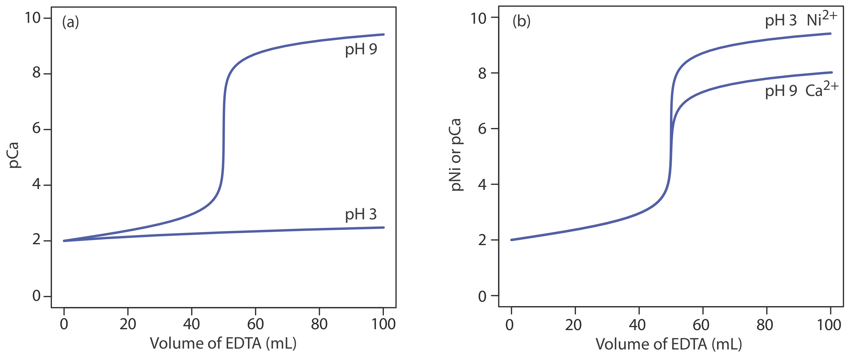
The scale of operations, accuracy, precision, sensitivity, time, and cost of a complexation titration are similar to those described earlier for acid–base titrations. Complexation titrations, however, are more selective. Although EDTA forms strong complexes with most metal ion, by carefully controlling the titrand’s pH we can analyze samples that contain two or more analytes. The reason we can use pH to provide selectivity is shown in Figure 9.3.9 a. A titration of Ca2+ at a pH of 9 has a distinct break in the titration curve because the conditional formation constant for CaY2– of \(2.6 \times 10^9\) is large enough to ensure that the reaction of Ca2+ and EDTA goes to completion. At a pH of 3, however, the conditional formation constant of 1.23 is so small that very little Ca2+ reacts with the EDTA. Suppose we need to analyze a mixture of Ni2+ and Ca2+. Both analytes react with EDTA, but their conditional formation constants differ significantly. If we adjust the pH to 3 we can titrate Ni2+ with EDTA without titrating Ca2+ (Figure 9.3.9 b). When the titration is complete, we adjust the titrand’s pH to 9 and titrate the Ca2+ with EDTA.
A spectrophotometric titration is a particularly useful approach for analyzing a mixture of analytes. For example, as shown in Figure 9.3.10 , we can determine the concentration of a two metal ions if there is a difference between the absorbance of the two metal-ligand complexes.