7.1: The Importance of Sampling
- Page ID
- 162880
\( \newcommand{\vecs}[1]{\overset { \scriptstyle \rightharpoonup} {\mathbf{#1}} } \)
\( \newcommand{\vecd}[1]{\overset{-\!-\!\rightharpoonup}{\vphantom{a}\smash {#1}}} \)
\( \newcommand{\id}{\mathrm{id}}\) \( \newcommand{\Span}{\mathrm{span}}\)
( \newcommand{\kernel}{\mathrm{null}\,}\) \( \newcommand{\range}{\mathrm{range}\,}\)
\( \newcommand{\RealPart}{\mathrm{Re}}\) \( \newcommand{\ImaginaryPart}{\mathrm{Im}}\)
\( \newcommand{\Argument}{\mathrm{Arg}}\) \( \newcommand{\norm}[1]{\| #1 \|}\)
\( \newcommand{\inner}[2]{\langle #1, #2 \rangle}\)
\( \newcommand{\Span}{\mathrm{span}}\)
\( \newcommand{\id}{\mathrm{id}}\)
\( \newcommand{\Span}{\mathrm{span}}\)
\( \newcommand{\kernel}{\mathrm{null}\,}\)
\( \newcommand{\range}{\mathrm{range}\,}\)
\( \newcommand{\RealPart}{\mathrm{Re}}\)
\( \newcommand{\ImaginaryPart}{\mathrm{Im}}\)
\( \newcommand{\Argument}{\mathrm{Arg}}\)
\( \newcommand{\norm}[1]{\| #1 \|}\)
\( \newcommand{\inner}[2]{\langle #1, #2 \rangle}\)
\( \newcommand{\Span}{\mathrm{span}}\) \( \newcommand{\AA}{\unicode[.8,0]{x212B}}\)
\( \newcommand{\vectorA}[1]{\vec{#1}} % arrow\)
\( \newcommand{\vectorAt}[1]{\vec{\text{#1}}} % arrow\)
\( \newcommand{\vectorB}[1]{\overset { \scriptstyle \rightharpoonup} {\mathbf{#1}} } \)
\( \newcommand{\vectorC}[1]{\textbf{#1}} \)
\( \newcommand{\vectorD}[1]{\overrightarrow{#1}} \)
\( \newcommand{\vectorDt}[1]{\overrightarrow{\text{#1}}} \)
\( \newcommand{\vectE}[1]{\overset{-\!-\!\rightharpoonup}{\vphantom{a}\smash{\mathbf {#1}}}} \)
\( \newcommand{\vecs}[1]{\overset { \scriptstyle \rightharpoonup} {\mathbf{#1}} } \)
\( \newcommand{\vecd}[1]{\overset{-\!-\!\rightharpoonup}{\vphantom{a}\smash {#1}}} \)
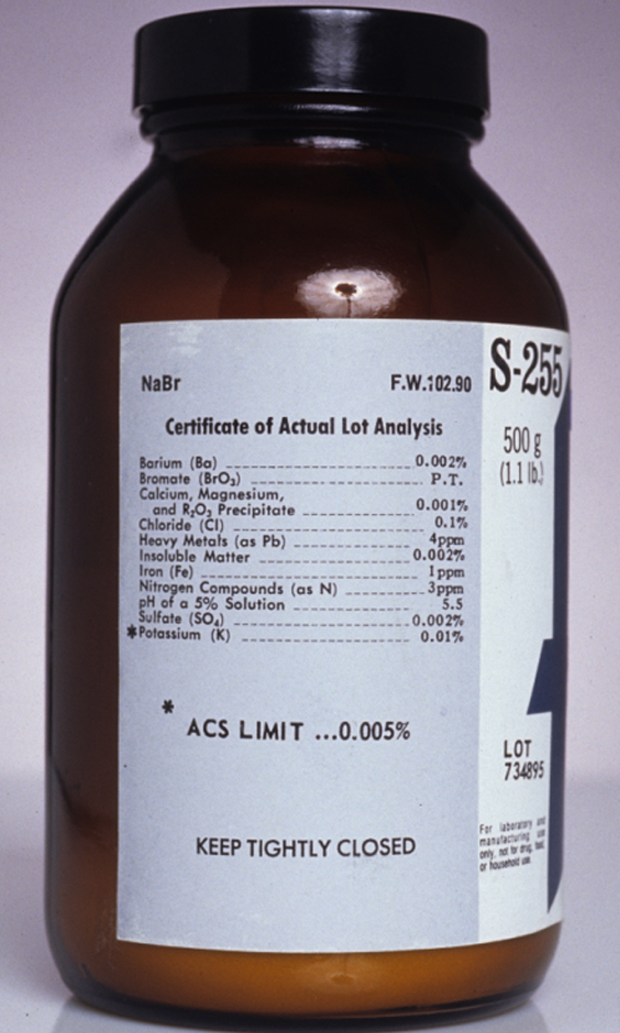
\(\newcommand{\avec}{\mathbf a}\) \(\newcommand{\bvec}{\mathbf b}\) \(\newcommand{\cvec}{\mathbf c}\) \(\newcommand{\dvec}{\mathbf d}\) \(\newcommand{\dtil}{\widetilde{\mathbf d}}\) \(\newcommand{\evec}{\mathbf e}\) \(\newcommand{\fvec}{\mathbf f}\) \(\newcommand{\nvec}{\mathbf n}\) \(\newcommand{\pvec}{\mathbf p}\) \(\newcommand{\qvec}{\mathbf q}\) \(\newcommand{\svec}{\mathbf s}\) \(\newcommand{\tvec}{\mathbf t}\) \(\newcommand{\uvec}{\mathbf u}\) \(\newcommand{\vvec}{\mathbf v}\) \(\newcommand{\wvec}{\mathbf w}\) \(\newcommand{\xvec}{\mathbf x}\) \(\newcommand{\yvec}{\mathbf y}\) \(\newcommand{\zvec}{\mathbf z}\) \(\newcommand{\rvec}{\mathbf r}\) \(\newcommand{\mvec}{\mathbf m}\) \(\newcommand{\zerovec}{\mathbf 0}\) \(\newcommand{\onevec}{\mathbf 1}\) \(\newcommand{\real}{\mathbb R}\) \(\newcommand{\twovec}[2]{\left[\begin{array}{r}#1 \\ #2 \end{array}\right]}\) \(\newcommand{\ctwovec}[2]{\left[\begin{array}{c}#1 \\ #2 \end{array}\right]}\) \(\newcommand{\threevec}[3]{\left[\begin{array}{r}#1 \\ #2 \\ #3 \end{array}\right]}\) \(\newcommand{\cthreevec}[3]{\left[\begin{array}{c}#1 \\ #2 \\ #3 \end{array}\right]}\) \(\newcommand{\fourvec}[4]{\left[\begin{array}{r}#1 \\ #2 \\ #3 \\ #4 \end{array}\right]}\) \(\newcommand{\cfourvec}[4]{\left[\begin{array}{c}#1 \\ #2 \\ #3 \\ #4 \end{array}\right]}\) \(\newcommand{\fivevec}[5]{\left[\begin{array}{r}#1 \\ #2 \\ #3 \\ #4 \\ #5 \\ \end{array}\right]}\) \(\newcommand{\cfivevec}[5]{\left[\begin{array}{c}#1 \\ #2 \\ #3 \\ #4 \\ #5 \\ \end{array}\right]}\) \(\newcommand{\mattwo}[4]{\left[\begin{array}{rr}#1 \amp #2 \\ #3 \amp #4 \\ \end{array}\right]}\) \(\newcommand{\laspan}[1]{\text{Span}\{#1\}}\) \(\newcommand{\bcal}{\cal B}\) \(\newcommand{\ccal}{\cal C}\) \(\newcommand{\scal}{\cal S}\) \(\newcommand{\wcal}{\cal W}\) \(\newcommand{\ecal}{\cal E}\) \(\newcommand{\coords}[2]{\left\{#1\right\}_{#2}}\) \(\newcommand{\gray}[1]{\color{gray}{#1}}\) \(\newcommand{\lgray}[1]{\color{lightgray}{#1}}\) \(\newcommand{\rank}{\operatorname{rank}}\) \(\newcommand{\row}{\text{Row}}\) \(\newcommand{\col}{\text{Col}}\) \(\renewcommand{\row}{\text{Row}}\) \(\newcommand{\nul}{\text{Nul}}\) \(\newcommand{\var}{\text{Var}}\) \(\newcommand{\corr}{\text{corr}}\) \(\newcommand{\len}[1]{\left|#1\right|}\) \(\newcommand{\bbar}{\overline{\bvec}}\) \(\newcommand{\bhat}{\widehat{\bvec}}\) \(\newcommand{\bperp}{\bvec^\perp}\) \(\newcommand{\xhat}{\widehat{\xvec}}\) \(\newcommand{\vhat}{\widehat{\vvec}}\) \(\newcommand{\uhat}{\widehat{\uvec}}\) \(\newcommand{\what}{\widehat{\wvec}}\) \(\newcommand{\Sighat}{\widehat{\Sigma}}\) \(\newcommand{\lt}{<}\) \(\newcommand{\gt}{>}\) \(\newcommand{\amp}{&}\) \(\definecolor{fillinmathshade}{gray}{0.9}\)When a manufacturer lists a chemical as ACS Reagent Grade, they must demonstrate that it conforms to specifications set by the American Chemical Society (ACS). For example, the ACS specifications for commercial NaBr require that the concentration of iron is less than 5 ppm. To verify that a production lot meets this standard, the manufacturer collects and analyzes several samples, reporting the average result on the product’s label (Figure 7.1.1 ).

If the individual samples do not represent accurately the population from which they are drawn—a population that we call the target population—then even a careful analysis will yield an inaccurate result. Extrapolating a result from a sample to its target population always introduces a determinate sampling error. To minimize this determinate sampling error, we must collect the right sample.
Even if we collect the right sample, indeterminate sampling errors may limit the usefulness of our analysis. Equation \ref{7.1} shows that a confidence interval about the mean, \(\overline{X}\) , is proportional to the standard deviation, s, of the analysis
\[\mu=\overline{X} \pm \frac{t s}{\sqrt{n}} \label{7.1}\]
where n is the number of samples and t is a statistical factor that accounts for the probability that the confidence interval contains the true value, \(\mu\).
Equation \ref{7.1} should be familiar to you. See Chapter 4 to review confidence intervals and see Appendix 4 for values of t.
Each step of an analysis contributes random error that affects the overall standard deviation. For convenience, let’s divide an analysis into two steps—collecting the samples and analyzing the samples—each of which is characterized by a variance. Using a propagation of uncertainty, the relationship between the overall variance, s2, and the variances due to sampling, \(s_{samp}^2\), and the variance due to the analytical method, \(s_{meth}^2\), is
\[s^{2}=s_{samp}^{2}+s_{meth}^{2} \label{7.2}\]
Although Equation \ref{7.1} is written in terms of a standard deviation, s, a propagation of uncertainty is written in terms of variances, s2. In this section, and those that follow, we will use both standard deviations and variances to discuss sampling uncertainty. For a review of the propagation of uncertainty, see Chapter 4.3 and Appendix 2.
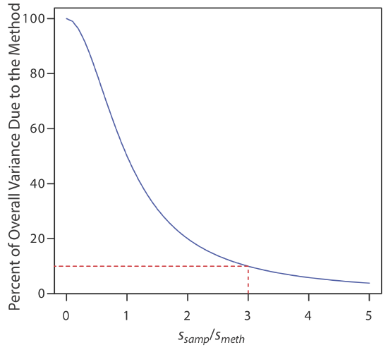
Equation \ref{7.2} shows that the overall variance for an analysis is limited by either the analytical method or sampling, or by both. Unfortunately, analysts often try to minimize the overall variance by improving only the method’s precision. This is a futile effort, however, if the standard deviation for sampling is more than three times greater than that for the method [Youden, Y. J. J. Assoc. Off. Anal. Chem. 1981, 50, 1007–1013]. Figure 7.1.2 shows how the ratio ssamp/smeth affects the method’s contribution to the overall variance. As shown by the dashed line, if the sample’s standard deviation is \(3 \times\) the method’s standard deviation, then indeterminate method errors explain only 10% of the overall variance. If indeterminate sampling errors are significant, decreasing smeth provides only limited improvement in the overall precision.

A quantitative analysis gives a mean concentration of 12.6 ppm for an analyte. The method’s standard deviation is 1.1 ppm and the standard deviation for sampling is 2.1 ppm. (a) What is the overall variance for the analysis? (b) By how much does the overall variance change if we improve smeth by 10% to 0.99 ppm? (c) By how much does the overall variance change if we improve ssamp by 10% to 1.9 ppm?
Solution
(a) The overall variance is
\[s^{2}=s_{samp}^{2}+s_{meth}^{2}=(2.1 \ \mathrm{ppm})^{2}+(1.1 \ \mathrm{ppm})^{2}=5.6 \ \mathrm{ppm}^{2} \nonumber\]
(b) Improving the method’s standard deviation changes the overall variance to
\[s^{2}=(2.1 \ \mathrm{ppm})^{2}+(0.99 \ \mathrm{ppm})^{2}=5.4 \ \mathrm{ppm}^{2} \nonumber\]
Improving the method’s standard deviation by 10% improves the overall variance by approximately 4%.
(c) Changing the standard deviation for sampling
\[s^{2}=(1.9 \ \mathrm{ppm})^{2}+(1.1 \ \mathrm{ppm})^{2}=4.8 \ \mathrm{ppm}^{2} \nonumber\]
improves the overall variance by almost 15%. As expected, because ssamp is larger than smeth, we achieve a bigger improvement in the overall variance when we focus our attention on sampling problems.
Suppose you wish to reduce the overall variance in Example 7.1.1 to 5.0 ppm2. If you focus on the method, by what percentage do you need to reduce smeth? If you focus on the sampling, by what percentage do you need to reduce ssamp?
- Answer
-
To reduce the overall variance by improving the method’s standard deviation requires that
\[s^{2}=5.00 \ \mathrm{ppm}^{2} = s_{samp}^{2}+s_{m e t h}^{2} = (2.1 \mathrm{ppm})^{2}+s_{m e t h}^{2} \nonumber\]
Solving for smeth gives its value as 0.768 ppm. Relative to its original value of 1.1 ppm, this is a reduction of \(3.0 \times 10^1\)%. To reduce the overall variance by improving the standard deviation for sampling requires that
\[s^{2}=5.00 \ \mathrm{ppm}^{2} = s_{samp}^{2}+s_{meth}^{2} = s_{samp}^{2}+(1.1 \ \mathrm{ppm})^{2} \nonumber\]
Solving for ssamp gives its value as 1.95 ppm. Relative to its original value of 2.1 ppm, this is reduction of 7.1%.
To determine which step has the greatest effect on the overall variance, we need to measure both ssamp and smeth. The analysis of replicate samples provides an estimate of the overall variance. To determine the method’s variance we must analyze samples under conditions where we can assume that the sampling variance is negligible; the sampling variance is then determined by difference.
There are several ways to minimize the standard deviation for sampling. Here are two examples. One approach is to use a standard reference material (SRM) that has been carefully prepared to minimize indeterminate sampling errors. When the sample is homogeneous—as is the case, for example, with an aqueous sample—then another useful approach is to conduct replicate analyses on a single sample.
The following data were collected as part of a study to determine the effect of sampling variance on the analysis of drug-animal feed formulations [Fricke, G. H.; Mischler, P. G.; Staffieri, F. P.; Houmyer, C. L. Anal. Chem. 1987, 59, 1213– 1217].
| % drug (w/w) | % drug (w/w) | ||||
|---|---|---|---|---|---|
| 0.0114 | 0.0099 | 0.0105 | 0.0105 | 0.0109 | 0.0107 |
| 0.0102 | 0.0106 | 0.0087 | 0.0103 | 0.0103 | 0.0104 |
| 0.0100 | 0.0095 | 0.0098 | 0.0101 | 0.0101 | 0.013 |
| 0.0105 | 0.0095 | 0.0097 | |||
The data on the left were obtained under conditions where both ssamp and smeth contribute to the overall variance. The data on the right were obtained under conditions where ssamp is insignificant. Determine the overall variance, and the standard deviations due to sampling and the analytical method. To which source of indeterminate error—sampling or the method—should we turn our attention if we want to improve the precision of the analysis?
Solution
Using the data on the left, the overall variance, s2, is \(4.71 \times 10^{-7}\). To find the method’s contribution to the overall variance, \(s_{meth}^2\), we use the data on the right, obtaining a value of \(7.00 \times 10^{-8}\). The variance due to sampling, \(s_{samp}^2\), is
\[s_{samp}^{2}=s^{2}-s_{meth}^{2} = 4.71 \times 10^{-7}-7.00 \times 10^{-8}=4.01 \times 10^{-7} \nonumber\]
Converting variances to standard deviations gives ssamp as \(6.33 \times 10^{-4}\) and smeth as \(2.65 \times 10^{-4}\). Because ssamp is more than twice as large as smeth, improving the precision of the sampling process will have the greatest impact on the overall precision.
A polymer’s density provides a measure of its crystallinity. The standard deviation for the determination of density using a single sample of a polymer is \(1.96 \times 10^{-3}\) g/cm3. The standard deviation when using different samples of the polymer is \(3.65 \times 10^{-2}\) g/cm3. Determine the standard deviations due to sampling and to the analytical method.
- Answer
-
The analytical method’s standard deviation is \(1.96 \times 10^{-3}\) g/cm3 as this is the standard deviation for the analysis of a single sample of the polymer. The sampling variance is
\[s_{sa m p}^{2}=s^{2}-s_{meth}^{2}= \left(3.65 \times 10^{-2}\right)^{2}-\left(1.96 \times 10^{-3}\right)^{2}=1.33 \times 10^{-3} \nonumber\]
Converting the variance to a standard deviation gives smeth as \(3.64 \times 10^{-2}\) g/cm3.


