
7.2: Designing a Sampling Plan
- Page ID
- 162881

\( \newcommand{\vecs}[1]{\overset { \scriptstyle \rightharpoonup} {\mathbf{#1}} } \)
\( \newcommand{\vecd}[1]{\overset{-\!-\!\rightharpoonup}{\vphantom{a}\smash {#1}}} \)
\( \newcommand{\id}{\mathrm{id}}\) \( \newcommand{\Span}{\mathrm{span}}\)
( \newcommand{\kernel}{\mathrm{null}\,}\) \( \newcommand{\range}{\mathrm{range}\,}\)
\( \newcommand{\RealPart}{\mathrm{Re}}\) \( \newcommand{\ImaginaryPart}{\mathrm{Im}}\)
\( \newcommand{\Argument}{\mathrm{Arg}}\) \( \newcommand{\norm}[1]{\| #1 \|}\)
\( \newcommand{\inner}[2]{\langle #1, #2 \rangle}\)
\( \newcommand{\Span}{\mathrm{span}}\)
\( \newcommand{\id}{\mathrm{id}}\)
\( \newcommand{\Span}{\mathrm{span}}\)
\( \newcommand{\kernel}{\mathrm{null}\,}\)
\( \newcommand{\range}{\mathrm{range}\,}\)
\( \newcommand{\RealPart}{\mathrm{Re}}\)
\( \newcommand{\ImaginaryPart}{\mathrm{Im}}\)
\( \newcommand{\Argument}{\mathrm{Arg}}\)
\( \newcommand{\norm}[1]{\| #1 \|}\)
\( \newcommand{\inner}[2]{\langle #1, #2 \rangle}\)
\( \newcommand{\Span}{\mathrm{span}}\) \( \newcommand{\AA}{\unicode[.8,0]{x212B}}\)
\( \newcommand{\vectorA}[1]{\vec{#1}} % arrow\)
\( \newcommand{\vectorAt}[1]{\vec{\text{#1}}} % arrow\)
\( \newcommand{\vectorB}[1]{\overset { \scriptstyle \rightharpoonup} {\mathbf{#1}} } \)
\( \newcommand{\vectorC}[1]{\textbf{#1}} \)
\( \newcommand{\vectorD}[1]{\overrightarrow{#1}} \)
\( \newcommand{\vectorDt}[1]{\overrightarrow{\text{#1}}} \)
\( \newcommand{\vectE}[1]{\overset{-\!-\!\rightharpoonup}{\vphantom{a}\smash{\mathbf {#1}}}} \)
\( \newcommand{\vecs}[1]{\overset { \scriptstyle \rightharpoonup} {\mathbf{#1}} } \)
\( \newcommand{\vecd}[1]{\overset{-\!-\!\rightharpoonup}{\vphantom{a}\smash {#1}}} \)
\(\newcommand{\avec}{\mathbf a}\) \(\newcommand{\bvec}{\mathbf b}\) \(\newcommand{\cvec}{\mathbf c}\) \(\newcommand{\dvec}{\mathbf d}\) \(\newcommand{\dtil}{\widetilde{\mathbf d}}\) \(\newcommand{\evec}{\mathbf e}\) \(\newcommand{\fvec}{\mathbf f}\) \(\newcommand{\nvec}{\mathbf n}\) \(\newcommand{\pvec}{\mathbf p}\) \(\newcommand{\qvec}{\mathbf q}\) \(\newcommand{\svec}{\mathbf s}\) \(\newcommand{\tvec}{\mathbf t}\) \(\newcommand{\uvec}{\mathbf u}\) \(\newcommand{\vvec}{\mathbf v}\) \(\newcommand{\wvec}{\mathbf w}\) \(\newcommand{\xvec}{\mathbf x}\) \(\newcommand{\yvec}{\mathbf y}\) \(\newcommand{\zvec}{\mathbf z}\) \(\newcommand{\rvec}{\mathbf r}\) \(\newcommand{\mvec}{\mathbf m}\) \(\newcommand{\zerovec}{\mathbf 0}\) \(\newcommand{\onevec}{\mathbf 1}\) \(\newcommand{\real}{\mathbb R}\) \(\newcommand{\twovec}[2]{\left[\begin{array}{r}#1 \\ #2 \end{array}\right]}\) \(\newcommand{\ctwovec}[2]{\left[\begin{array}{c}#1 \\ #2 \end{array}\right]}\) \(\newcommand{\threevec}[3]{\left[\begin{array}{r}#1 \\ #2 \\ #3 \end{array}\right]}\) \(\newcommand{\cthreevec}[3]{\left[\begin{array}{c}#1 \\ #2 \\ #3 \end{array}\right]}\) \(\newcommand{\fourvec}[4]{\left[\begin{array}{r}#1 \\ #2 \\ #3 \\ #4 \end{array}\right]}\) \(\newcommand{\cfourvec}[4]{\left[\begin{array}{c}#1 \\ #2 \\ #3 \\ #4 \end{array}\right]}\) \(\newcommand{\fivevec}[5]{\left[\begin{array}{r}#1 \\ #2 \\ #3 \\ #4 \\ #5 \\ \end{array}\right]}\) \(\newcommand{\cfivevec}[5]{\left[\begin{array}{c}#1 \\ #2 \\ #3 \\ #4 \\ #5 \\ \end{array}\right]}\) \(\newcommand{\mattwo}[4]{\left[\begin{array}{rr}#1 \amp #2 \\ #3 \amp #4 \\ \end{array}\right]}\) \(\newcommand{\laspan}[1]{\text{Span}\{#1\}}\) \(\newcommand{\bcal}{\cal B}\) \(\newcommand{\ccal}{\cal C}\) \(\newcommand{\scal}{\cal S}\) \(\newcommand{\wcal}{\cal W}\) \(\newcommand{\ecal}{\cal E}\) \(\newcommand{\coords}[2]{\left\{#1\right\}_{#2}}\) \(\newcommand{\gray}[1]{\color{gray}{#1}}\) \(\newcommand{\lgray}[1]{\color{lightgray}{#1}}\) \(\newcommand{\rank}{\operatorname{rank}}\) \(\newcommand{\row}{\text{Row}}\) \(\newcommand{\col}{\text{Col}}\) \(\renewcommand{\row}{\text{Row}}\) \(\newcommand{\nul}{\text{Nul}}\) \(\newcommand{\var}{\text{Var}}\) \(\newcommand{\corr}{\text{corr}}\) \(\newcommand{\len}[1]{\left|#1\right|}\) \(\newcommand{\bbar}{\overline{\bvec}}\) \(\newcommand{\bhat}{\widehat{\bvec}}\) \(\newcommand{\bperp}{\bvec^\perp}\) \(\newcommand{\xhat}{\widehat{\xvec}}\) \(\newcommand{\vhat}{\widehat{\vvec}}\) \(\newcommand{\uhat}{\widehat{\uvec}}\) \(\newcommand{\what}{\widehat{\wvec}}\) \(\newcommand{\Sighat}{\widehat{\Sigma}}\) \(\newcommand{\lt}{<}\) \(\newcommand{\gt}{>}\) \(\newcommand{\amp}{&}\) \(\definecolor{fillinmathshade}{gray}{0.9}\)A sampling plan must support the goals of an analysis. For example, a material scientist interested in characterizing a metal’s surface chemistry is more likely to choose a freshly exposed surface, created by cleaving the sample under vacuum, than a surface previously exposed to the atmosphere. In a qualitative analysis, a sample need not be identical to the original substance provided there is sufficient analyte present to ensure its detection. In fact, if the goal of an analysis is to identify a trace-level component, it may be desirable to discriminate against major components when collecting samples.
For an interesting discussion of the importance of a sampling plan, see Buger, J. et al. “Do Scientists and Fishermen Collect the Same Size Fish? Possible Implications for Exposure Assessment,” Environ. Res. 2006, 101, 34–41.
For a quantitative analysis, the sample’s composition must represent accurately the target population, a requirement that necessitates a careful sampling plan. Among the issues we need to consider are these five questions.
- From where within the target population should we collect samples?
- What type of samples should we collect?
- What is the minimum amount of sample needed for each analysis?
- How many samples should we analyze?
- How can we minimize the overall variance for the analysis?
Where to Sample the Target Population
A sampling error occurs whenever a sample’s composition is not identical to its target population. If the target population is homogeneous, then we can collect individual samples without giving consideration to where we collect sample. Unfortunately, in most situations the target population is heterogeneous and attention to where we collect samples is important. For example, due to settling a medication available as an oral suspension may have a higher concentration of its active ingredients at the bottom of the container. The composition of a clinical sample, such as blood or urine, may depend on when it is collected. A patient’s blood glucose level, for instance, will change in response to eating and exercise. Other target populations show both a spatial and a temporal heterogeneity. The concentration of dissolved O2 in a lake is heterogeneous due both to a change in seasons and to point sources of pollution.
The composition of a homogeneous target population is the same regardless of where we sample, when we sample, or the size of our sample. For a heterogeneous target population, the composition is not the same at different locations, at different times, or for different sample sizes.
If the analyte’s distribution within the target population is a concern, then our sampling plan must take this into account. When feasible, homogenizing the target population is a simple solution, although this often is impracticable. In addition, homogenizing a sample destroys information about the analyte’s spatial or temporal distribution within the target population, information that may be of importance.
Random Sampling
The ideal sampling plan provides an unbiased estimate of the target population’s properties. A random sampling is the easiest way to satisfy this requirement [Cohen, R. D. J. Chem. Educ. 1991, 68, 902–903]. Despite its apparent simplicity, a truly random sample is difficult to collect. Haphazard sampling, in which samples are collected without a sampling plan, is not random and may reflect an analyst’s unintentional biases.
Here is a simple method to ensure that we collect random samples. First, we divide the target population into equal units and assign to each unit a unique number. Then, we use a random number table to select the units to sample. Example 7.2.1 provides an illustrative example. Appendix 14 provides a random number table that you can use to design a sampling plan.
To analyze a polymer’s tensile strength, individual samples of the polymer are held between two clamps and stretched. To evaluate a production lot, the manufacturer’s sampling plan calls for collecting ten 1 cm \(\times\) 1 cm samples from a 100 cm \(\times\) 100 cm polymer sheet. Explain how we can use a random number table to ensure that we collect these samples at random.
Solution
As shown by the grid below, we divide the polymer sheet into 10 000 1 cm \(\times\) 1 cm squares, each identified by its row number and its column number, with numbers running from 0 to 99.
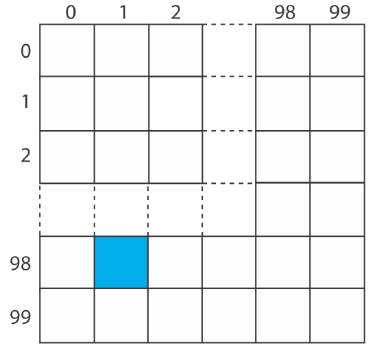
For example, the blue square is in row 98 and in column 1. To select ten squares at random, we enter the random number table in Appendix 14 at an arbitrary point and let the entry’s last four digits represent the row number and the column number for the first sample. We then move through the table in a predetermined fashion, selecting random numbers until we have 10 samples. For our first sample, let’s use the second entry in the third column of Appendix 14 , which is 76831. The first sample, therefore, is row 68 and column 31. If we proceed by moving down the third column, then the 10 samples are as follows:
| sample | number | row | column | sample | number | roq | column |
|---|---|---|---|---|---|---|---|
| 1 | 76831 | 68 | 31 | 6 | 41701 | 17 | 01 |
| 2 |
66558 |
65 | 58 | 7 | 38605 | 86 | 05 |
| 3 | 33266 | 32 | 66 | 8 | 64516 | 45 | 16 |
| 4 | 12032 | 20 | 32 | 9 | 13015 | 30 | 15 |
| 5 | 14063 | 40 | 63 | 10 | 12138 | 21 | 38 |
When we collect a random sample we make no assumptions about the target population, which makes this the least biased approach to sampling. On the other hand, a random sample often requires more time and expense than other sampling strategies because we need to collect a greater number of samples to ensure that we adequately sample the target population, particularly when that population is heterogenous [Borgman, L. E.; Quimby, W. F. in Keith, L. H., ed. Principles of Environmental Sampling, American Chemical Society: Washington, D. C., 1988, 25–43].
Judgmental Sampling
The opposite of random sampling is selective, or judgmental sampling in which we use prior information about the target population to help guide our selection of samples. Judgmental sampling is more biased than random sampling, but requires fewer samples. Judgmental sampling is useful if we wish to limit the number of independent variables that might affect our results. For example, if we are studying the bioaccumulation of PCB’s in fish, we may choose to exclude fish that are too small, too young, or that appear diseased.
Systematic Sampling
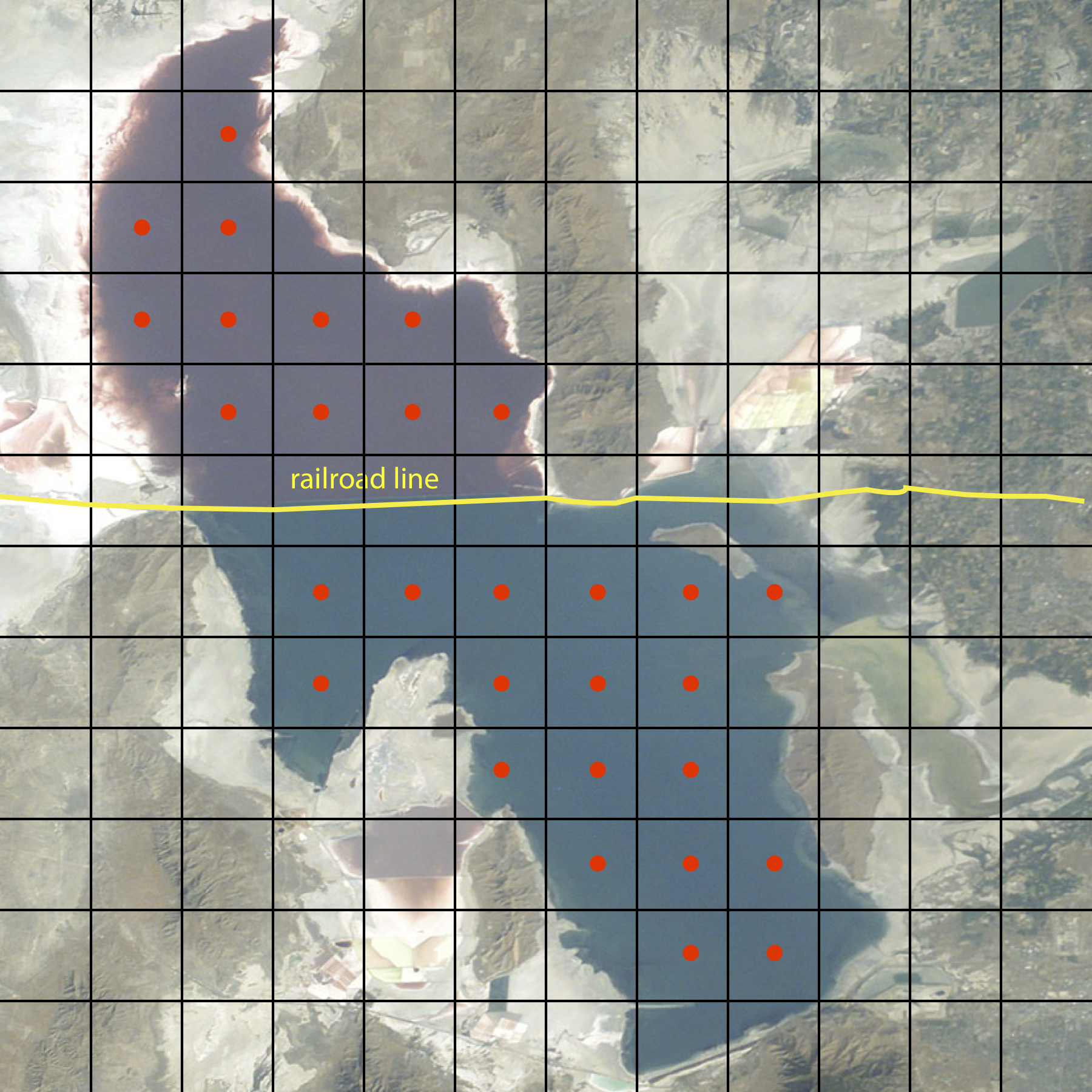
Random sampling and judgmental sampling represent extremes in bias and in the number of samples needed to characterize the target population. Systematic sampling falls in between these extremes. In systematic sampling we sample the target population at regular intervals in space or time. Figure 7.2.1 shows an aerial photo of the Great Salt Lake in Utah. A railroad line divides the lake into two sections that have different chemical compositions. To compare the lake’s two sections—and to evaluate spatial variations within each section—we use a two-dimensional grid to define sampling locations, collecting samples at the center of each location. When a population’s is heterogeneous in time, as is common in clinical and environmental studies, then we might choose to collect samples at regular intervals in time.
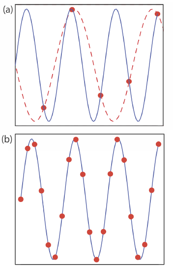
If a target population’s properties have a periodic trend, a systematic sampling will lead to a significant bias if our sampling frequency is too small. This is a common problem when sampling electronic signals where the problem is known as aliasing. Consider, for example, a signal that is a simple sign wave. Figure 7.2.2 a shows how an insufficient sampling frequency underestimates the signal’s true frequency. The apparent signal, shown by the dashed red line that passes through the five data points, is significantly different from the true signal shown by the solid blue line.
According to the Nyquist theorem, to determine accurately the frequency of a periodic signal, we must sample the signal at least twice during each cycle or period. If we collect samples at an interval of \(\Delta t\), then the highest frequency we can monitor accurately is \((2 \Delta t)^{-1}\). For example, if we collect one sample each hour, then the highest frequency we can monitor is (2 \(\times\) 1 hr)–1 or 0.5 hr–1, a period of less than 2 hr. If our signal’s period is less than 2 hours (a frequency of more than 0.5 hr–1), then we must use a faster sampling rate. Ideally, we use a sampling rate that is at least 3–4 times greater than the highest frequency signal of interest. If our signal has a period of one hour, then we should collect a new sample every 15-20 minutes.
Systematic–Judgmental Sampling
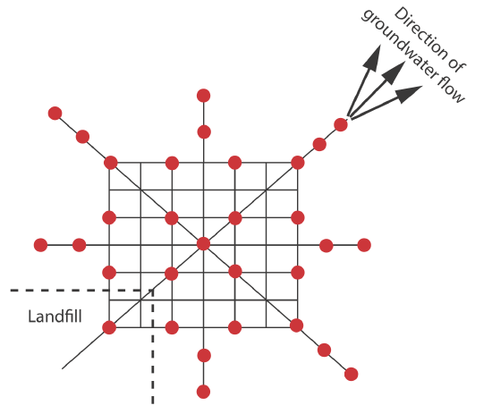
Combinations of the three primary approaches to sampling also are possible [Keith, L. H. Environ. Sci. Technol. 1990, 24, 610–617]. One such combination is systematic–judgmental sampling, in which we use prior knowledge about a system to guide a systematic sampling plan. For example, when monitoring waste leaching from a landfill, we expect the plume to move in the same direction as the flow of groundwater—this helps focus our sampling, saving money and time. The systematic–judgmental sampling plan in Figure 7.2.3 includes a rectangular grid for most of the samples and linear transects to explore the plume’s limits [Flatman, G. T.; Englund, E. J.; Yfantis, A. A. in Keith, L. H., ed. Principles of Environmental Sampling, American Chemical Society: Washington, D. C., 1988, 73–84].
Stratified Sampling
Another combination of the three primary approaches to sampling is judgmental–random, or stratified sampling. Many target populations consist of distinct units, or strata. For example, suppose we are studying particulate Pb in urban air. Because particulates come in a range of sizes—some visible and some microscopic—and come from many sources—such as road dust, diesel soot, and fly ash to name a few—we can subdivide the target population by size or by source. If we choose a random sampling plan, then we collect samples without considering the different strata, which may bias the sample toward larger particulates. In a stratified sampling we divide the target population into strata and collect random samples from within each stratum. After we analyze the samples from each stratum, we pool their respective means to give an overall mean for the target population. The advantage of stratified sampling is that individual strata usually are more homogeneous than the target population. The overall sampling variance for stratified sampling always is at least as good, and often is better than that obtained by simple random sampling. Because a stratified sampling requires that we collect and analyze samples from several strata, it often requires more time and money.
Convenience Sampling
One additional method of sampling deserves mention. In convenience sampling we select sample sites using criteria other than minimizing sampling error and sampling variance. In a survey of rural groundwater quality, for example, we can choose to drill wells at sites selected at random or we can choose to take advantage of existing wells; the latter usually is the preferred choice. In this case cost, expedience, and accessibility are more important than ensuring a random sample
What Type of Sample to Collect
Having determined from where to collect samples, the next step in designing a sampling plan is to decide on the type of sample to collect. There are three common methods for obtaining samples: grab sampling, composite sampling, and in situ sampling.
The most common type of sample is a grab sample in which we collect a portion of the target population at a specific time or location, providing a “snapshot” of the target population. If our target population is homogeneous, a series of random grab samples allows us to establish its properties. For a heterogeneous target population, systematic grab sampling allows us to characterize how its properties change over time and/or space.
A composite sample is a set of grab samples that we combine into a single sample before analysis. Because information is lost when we combine individual samples, normally we analyze separately each grab sample. In some situations, however, there are advantages to working with a composite sample.
One situation where composite sampling is appropriate is when our interest is in the target population’s average composition over time or space. For example, wastewater treatment plants must monitor and report the average daily composition of the treated water they release to the environment. The analyst can collect and analyze a set of individual grab samples and report the average result, or she can save time and money by combining the grab samples into a single composite sample and report the result of her analysis of the composite sample.
Composite sampling also is useful when a single sample does not supply sufficient material for the analysis. For example, analytical methods for the quantitative analysis of PCB’s in fish often require as much as 50 g of tissue, an amount that may be difficult to obtain from a single fish. Combining and homogenizing tissue samples from several fish makes it easy to obtain the necessary 50-g sample.
A significant disadvantage of grab samples and composite samples is that we cannot use them to monitor continuously a time-dependent change in the target population. In situ sampling, in which we insert an analytical sensor into the target population, allows us to monitor the target population without removing individual grab samples. For example, we can monitor the pH of a solution in an industrial production line by immersing a pH electrode in the solution’s flow.
A study of the relationship between traffic density and the concentrations of Pb, Cd, and Zn in roadside soils uses the following sampling plan [Nabulo, G.; Oryem-Origa, H.; Diamond, M. Environ. Res. 2006, 101, 42–52]. Samples of surface soil (0–10 cm) are collected at distances of 1, 5, 10, 20, and 30 m from the road. At each distance, 10 samples are taken from different locations and mixed to form a single sample. What type of sampling plan is this? Explain why this is an appropriate sampling plan.
Solution
This is a systematic–judgemental sampling plan using composite samples. These are good choices given the goals of the study. Automobile emissions release particulates that contain elevated concentrations of Pb, Cd, and Zn—this study was conducted in Uganda where leaded gasoline was still in use—which settle out on the surrounding roadside soils as “dry rain.” Samples collected near the road and samples collected at fixed distances from the road provide sufficient data for the study, while minimizing the total number of samples. Combining samples from the same distance into a single, composite sample has the advantage of decreasing sampling uncertainty.
How Much Sample to Collect
To minimize sampling errors, samples must be of an appropriate size. If a sample is too small its composition may differ substantially from that of the target population, which introduces a sampling error. Samples that are too large, however, require more time and money to collect and analyze, without providing a significant improvement in the sampling error.
Let’s assume our target population is a homogeneous mixture of two types of particles. Particles of type A contain a fixed concentration of analyte, and particles of type B are analyte-free. Samples from this target population follow a binomial distribution. If we collect a sample of n particles, then the expected number of particles that contains analyte, nA, is
\[n_{A}=n p \nonumber\]
where p is the probability of selecting a particle of type A. The standard deviation for sampling is
\[s_{samp}=\sqrt{n p(1-p)} \label{7.1}\]
To calculate the relative standard deviation for sampling, \(\left( s_{samp} \right)_{rel}\), we divide Equation \ref{7.1} by nA, obtaining
\[\left(s_{samp}\right)_{r e l}=\frac{\sqrt{n p(1-p)}}{n p} \nonumber\]
Solving for n allows us to calculate the number of particles we need to provide a desired relative sampling variance.
\[n=\frac{1-p}{p} \times \frac{1}{\left(s_{s a m p}\right)_{rel}^{2}} \label{7.2}\]
Suppose we are analyzing a soil where the particles that contain analyte represent only \(1 \times 10^{-7}\)% of the population. How many particles must we collect to give a percent relative standard deviation for sampling of 1%?
Solution
Since the particles of interest account for \(1 \times 10^{-7}\)% of all particles, the probability, p, of selecting one of these particles is \(1 \times 10^{-9}\). Substituting into Equation \ref{7.2} gives
\[n=\frac{1-\left(1 \times 10^{-9}\right)}{1 \times 10^{-9}} \times \frac{1}{(0.01)^{2}}=1 \times 10^{13} \nonumber\]
To obtain a relative standard deviation for sampling of 1%, we need to collect \(1 \times 10^{13}\) particles.
Depending on the particle size, a sample of 1013 particles may be fairly large. Suppose this is equivalent to a mass of 80 g. Working with a sample this large clearly is not practical. Does this mean we must work with a smaller sample and accept a larger relative standard deviation for sampling? Fortunately the answer is no. An important feature of Equation \ref{7.2} is that the relative standard deviation for sampling is a function of the number of particles instead of their combined mass. If we crush and grind the particles to make them smaller, then a sample of 1013 particles will have a smaller mass. If we assume that a particle is spherical, then its mass is proportional to the cube of its radius.
\[\operatorname{mass} \propto r^{3} \nonumber\]
If we decrease a particle’s radius by a factor of 2, for example, then we decrease its mass by a factor of 23, or 8. This assumes, of course, that the process of crushing and grinding particles does not change the composition of the particles.
Assume that a sample of 1013 particles from Example 7.2.3 weighs 80 g and that the particles are spherical. By how much must we reduce a particle’s radius if we wish to work with 0.6-g samples?
Solution
To reduce the sample’s mass from 80 g to 0.6 g, we must change its mass by a factor of
\[\frac{80}{0.6}=133 \times \nonumber\]
To accomplish this we must decrease a particle’s radius by a factor of
\[\begin{aligned} r^{3} &=133 \times \\ r &=5.1 \times \end{aligned} \nonumber\]
Decreasing the radius by a factor of approximately 5 allows us to decrease the sample’s mass from 80 g to 0.6 g.
Treating a population as though it contains only two types of particles is a useful exercise because it shows us that we can improve the relative standard deviation for sampling by collecting more particles. Of course, a real population likely contains more than two types of particles, with the analyte present at several levels of concentration. Nevertheless, the sampling of many well-mixed populations approximate binomial sampling statistics because they are homogeneous on the scale at which they are sampled. Under these conditions the following relationship between the mass of a random grab sample, m, and the percent relative standard deviation for sampling, R, often is valid
where Ks is a sampling constant equal to the mass of a sample that produces a percent relative standard deviation for sampling of ±1% [Ingamells, C. O.; Switzer, P. Talanta 1973, 20, 547–568].
The following data were obtained in a preliminary determination of the amount of inorganic ash in a breakfast cereal.
| mass of cereal (g) | 0.9956 | 0.9981 | 1.0036 | 0.9994 | 1.0067 |
| %w/w ash | 1.34 | 1.29 | 1.32 | 1.26 | 1.28 |
What is the value of Ks and what size sample is needed to give a percent relative standard deviation for sampling of ±2.0%. Predict the percent relative standard deviation and the absolute standard deviation if we collect 5.00-g samples.
Solution
To determine the sampling constant, Ks, we need to know the average mass of the cereal samples and the relative standard deviation for the amount of ash in those samples. The average mass of the cereal samples is 1.0007 g. The average %w/w ash and its absolute standard deviation are, respectively, 1.298 %w/w and 0.03194 %w/w. The percent relative standard deviation, R, therefore, is
\[R=\frac{s_{\text { samp }}}{\overline{X}}=\frac{0.03194 \% \ \mathrm{w} / \mathrm{w}}{1.298 \% \ \mathrm{w} / \mathrm{w}} \times 100=2.46 \% \nonumber\]
Solving for Ks gives its value as
\[K_{s}=m R^{2}=(1.0007 \mathrm{g})(2.46)^{2}=6.06 \ \mathrm{g} \nonumber\]
To obtain a percent relative standard deviation of ±2%, samples must have a mass of at least
\[m=\frac{K_{s}}{R^{2}}=\frac{6.06 \mathrm{g}}{(2.0)^{2}}=1.5 \ \mathrm{g} \nonumber\]
If we use 5.00-g samples, then the expected percent relative standard deviation is
\[R=\sqrt{\frac{K_{s}}{m}}=\sqrt{\frac{6.06 \mathrm{g}}{5.00 \mathrm{g}}}=1.10 \% \nonumber\]
and the expected absolute standard deviation is
\[s_{\text { samp }}=\frac{R \overline{X}}{100}=\frac{(1.10)(1.298 \% \mathrm{w} / \mathrm{w})}{100}=0.0143 \% \mathrm{w} / \mathrm{w} \nonumber\]
Olaquindox is a synthetic growth promoter in medicated feeds for pigs. In an analysis of a production lot of feed, five samples with nominal masses of 0.95 g were collected and analyzed, with the results shown in the following table.
| mass (g) | 0.9530 | 0.9728 | 0.9660 | 0.9402 | 0.9576 |
| mg olaquindox/kg feed | 23.0 | 23.8 | 21.0 | 26.5 | 21.4 |
What is the value of Ks and what size samples are needed to obtain a percent relative deviation for sampling of 5.0%? By how much do you need to reduce the average particle size if samples must weigh no more than 1 g?
- Answer
-
To determine the sampling constant, Ks, we need to know the average mass of the samples and the percent relative standard deviation for the concentration of olaquindox in the feed. The average mass for the five samples is 0.95792 g. The average concentration of olaquindox in the samples is 23.14 mg/kg with a standard deviation of 2.200 mg/kg. The percent relative standard deviation, R, is
\[R=\frac{s_{\text { samp }}}{\overline{X}} \times 100=\frac{2.200 \ \mathrm{mg} / \mathrm{kg}}{23.14 \ \mathrm{mg} / \mathrm{kg}} \times 100=9.507 \approx 9.51 \nonumber\]
Solving for Ks gives its value as
\[K_{s}=m R^{2}=(0.95792 \mathrm{g})(9.507)^{2}=86.58 \ \mathrm{g} \approx 86.6 \ \mathrm{g} \nonumber\]
To obtain a percent relative standard deviation of 5.0%, individual samples need to have a mass of at least
\[m=\frac{K_{s}}{R^{2}}=\frac{86.58 \ \mathrm{g}}{(5.0)^{2}}=3.5 \ \mathrm{g} \nonumber\]
To reduce the sample’s mass from 3.5 g to 1 g, we must change the mass by a factor of
\[\frac{3.5 \ \mathrm{g}}{1 \ \mathrm{g}}=3.5 \times \nonumber\]
If we assume that the sample’s particles are spherical, then we must reduce a particle’s radius by a factor of
\[\begin{aligned} r^{3} &=3.5 \times \\ r &=1.5 \times \end{aligned} \nonumber\]
How Many Samples to Collect
In the previous section we considered how much sample we need to minimize the standard deviation due to sampling. Another important consideration is the number of samples to collect. If the results from our analysis of the samples are normally distributed, then the confidence interval for the sampling error is
\[\mu=\overline{X} \pm \frac{t s_{samp}}{\sqrt{n_{samp}}} \label{7.4}\]
where nsamp is the number of samples and ssamp is the standard deviation for sampling. Rearranging Equation \ref{7.4} and substituting e for the quantity \(\overline{X} - \mu\), gives the number of samples as
\[n_{samp}=\frac{t^{2} s_{samp}^{2}}{e^{2}} \label{7.5}\]
Because the value of t depends on nsamp, the solution to Equation \ref{7.5} is found iteratively.
When we use Equation \ref{7.5}, we must express the standard deviation for sampling, ssamp, and the error, e, in the same way. If ssamp is reported as a percent relative standard deviation, then the error, e, is reported as a percent relative error. When you use Equation \ref{7.5}, be sure to check that you are expressing ssamp and e in the same way.
In Example 7.2.5 we determined that we need 1.5-g samples to establish an ssamp of ±2.0% for the amount of inorganic ash in cereal. How many 1.5-g samples do we need to collect to obtain a percent relative sampling error of ±0.80% at the 95% confidence level?
Solution
Because the value of t depends on the number of samples—a result we have yet to calculate—we begin by letting nsamp = \(\infty\) and using t(0.05, \(\infty\)) for t. From Appendix 4, the value for t(0.05, \(\infty\)) is 1.960. Substituting known values into Equation \ref{7.5} gives the number of samples as
\[n_{samp}=\frac{(1.960)^{2}(2.0)^{2}}{(0.80)^{2}}=24.0 \approx 24 \nonumber\]
Letting nsamp = 24, the value of t(0.05, 23) from Appendix 4 is 2.073. Recalculating nsamp gives
\[n_{samp}=\frac{(2.073)^{2}(2.0)^{2}}{(0.80)^{2}}=26.9 \approx 27 \nonumber\]
When nsamp = 27, the value of t(0.05, 26) from Appendix 4 is 2.060. Recalculating nsamp gives
\[n_{samp}=\frac{(2.060)^{2}(2.0)^{2}}{(0.80)^{2}}=26.52 \approx 27 \nonumber\]
Because two successive calculations give the same value for nsamp, we have an iterative solution to the problem. We need 27 samples to achieve a percent relative sampling error of ±0.80% at the 95% confidence level.
Assuming that the percent relative standard deviation for sampling in the determination of olaquindox in medicated feed is 5.0% (see Exercise 7.2.1 ), how many samples do we need to analyze to obtain a percent relative sampling error of ±2.5% at \(\alpha\) = 0.05?
- Answer
-
Because the value of t depends on the number of samples—a result we have yet to calculate—we begin by letting nsamp = \(\infty\) and using t(0.05, \(\infty\)) for the value of t. From Appendix 4, the value for t(0.05, \(\infty\)) is 1.960. Our first estimate for nsamp is
\[n_{samp}=\frac{t^{2} s_{s a m p}^{2}}{e^{2}} = \frac{(1.96)^{2}(5.0)^{2}}{(2.5)^{2}}=15.4 \approx 15 \nonumber\]
Letting nsamp = 15, the value of t(0.05,14) from Appendix 4 is 2.145. Recalculating nsamp gives
\[n_{samp}=\frac{t^{2} s_{samp}^{2}}{e^{2}}=\frac{(2.145)^{2}(5.0)^{2}}{(2.5)^{2}}=18.4 \approx 18 \nonumber\]
Letting nsamp = 18, the value of t(0.05,17) from Appendix 4 is 2.103. Recalculating nsamp gives
\[n_{samp}=\frac{t^{2} s_{samp}^{2}}{e^{2}}=\frac{(2.103)^{2}(5.0)^{2}}{(2.5)^{2}}=17.7 \approx 18 \nonumber\]
Because two successive calculations give the same value for nsamp, we need 18 samples to achieve a sampling error of ±2.5% at the 95% confidence interval.
Equation \ref{7.5} provides an estimate for the smallest number of samples that will produce the desired sampling error. The actual sampling error may be substantially larger if ssamp for the samples we collect during the subsequent analysis is greater than ssamp used to calculate nsamp. This is not an uncommon problem. For a target population with a relative sampling variance of 50 and a desired relative sampling error of ±5%, Equation \ref{7.5} predicts that 10 samples are sufficient. In a simulation using 1000 samples of size 10, however, only 57% of the trials resulted in a sampling error of less than ±5% [Blackwood, L. G. Environ. Sci. Technol. 1991, 25, 1366–1367]. Increasing the number of samples to 17 was sufficient to ensure that the desired sampling error was achieved 95% of the time.
For an interesting discussion of why the number of samples is important, see Kaplan, D.; Lacetera, N.; Kaplan, C. “Sample Size and Precision in NIH Peer Review,” Plos One, 2008, 3(7), 1–3. When reviewing grants, individual reviewers report a score between 1.0 and 5.0 (two significant figures). NIH reports the average score to three significant figures, implying that a difference of 0.01 is significant. If the individual scores have a standard deviation of 0.1, then a difference of 0.01 is significant at \(\alpha = 0.05\) only if there are 384 reviews. The authors conclude that NIH review panels are too small to provide a statistically meaningful separation between proposals receiving similar scores.
Minimizing the Overall Variance
A final consideration when we develop a sampling plan is how we can minimize the overall variance for the analysis. Equation 7.1.2 shows that the overall variance is a function of the variance due to the method, \(s_{meth}^2\), and the variance due to sampling, \(s_{samp}^2\). As we learned earlier, we can improve the sampling variance by collecting more samples of the proper size. Increasing the number of times we analyze each sample improves the method’s variance. If \(s_{samp}^2\) is significantly greater than \(s_{meth}^2\), we can ignore the method’s contribution to the overall variance and use Equation \ref{7.5} to estimate the number of samples to analyze. Analyzing any sample more than once will not improve the overall variance, because the method’s variance is insignificant.
If \(s_{meth}^2\) is significantly greater than \(s_{samp}^2\), then we need to collect and analyze only one sample. The number of replicate analyses, nrep, we need to minimize the error due to the method is given by an equation similar to Equation \ref{7.5}.
\[n_{rep}=\frac{t^{2} s_{m e t h}^{2}}{e^{2}} \nonumber\]
Unfortunately, the simple situations described above often are the exception. For many analyses, both the sampling variance and the method variance are significant, and both multiple samples and replicate analyses of each sample are necessary. The overall error in this case is
\[e=t \sqrt{\frac{s_{samp}^{2}}{n_{samp}} + \frac{s_{meth}^{2}}{n_{sam p} n_{rep}}} \label{7.6}\]
Equation \ref{7.6} does not have a unique solution as different combinations of nsamp and nrep give the same overall error. How many samples we collect and how many times we analyze each sample is determined by other concerns, such as the cost of collecting and analyzing samples, and the amount of available sample.
An analytical method has a relative sampling variance of 0.40% and a relative method variance of 0.070%. Evaluate the percent relative error (\(\alpha = 0.05\)) if you collect 5 samples and analyze each twice, and if you collect 2 samples and analyze each 5 times.
Solution
Both sampling strategies require a total of 10 analyses. From Appendix 4 we find that the value of t(0.05, 9) is 2.262. Using Equation \ref{7.6}, the relative error for the first sampling strategy is
\[e=2.262 \sqrt{\frac{0.40}{5}+\frac{0.070}{5 \times 2}}=0.67 \% \nonumber\]
and that for the second sampling strategy is
\[e=2.262 \sqrt{\frac{0.40}{2}+\frac{0.070}{2 \times 5}}=1.0 \% \nonumber\]
Because the method variance is smaller than the sampling variance, we obtain a smaller relative error if we collect more samples and analyze each sample fewer times.
An analytical method has a relative sampling variance of 0.10% and a relative method variance of 0.20%. The cost of collecting a sample is $20 and the cost of analyzing a sample is $50. Propose a sampling strategy that provides a maximum relative error of ±0.50% (\(\alpha = 0.05\)) and a maximum cost of $700.
- Answer
-
If we collect a single sample (cost $20), then we can analyze that sample 13 times (cost $650) and stay within our budget. For this scenario, the percent relative error is
\[e=t \sqrt{\frac{s_{samp}^{2}}{n_{samp}} + \frac{s_{meth}^{2}}{n_{sam p} n_{rep}}} = 2.179 \sqrt{\frac{0.10}{1}+\frac{0.20}{1 \times 13}}=0.74 \% \nonumber\]
where t(0.05, 12) is 2.179. Because this percent relative error is larger than ±0.50%, this is not a suitable sampling strategy.
Next, we try two samples (cost $40), analyzing each six times (cost $600). For this scenario, the percent relative error is
\[e=t \sqrt{\frac{s_{samp}^{2}}{n_{samp}} + \frac{s_{meth}^{2}}{n_{sam p} n_{rep}}} = 2.2035 \sqrt{\frac{0.10}{2}+\frac{0.20}{2 \times 6}}=0.57 \% \nonumber\]
where t(0.05, 11) is 2.2035. Because this percent relative error is larger than ±0.50%, this also is not a suitable sampling strategy.
Next we try three samples (cost $60), analyzing each four times (cost $600). For this scenario, the percent relative error is
\[e=t \sqrt{\frac{s_{samp}^{2}}{n_{samp}} + \frac{s_{meth}^{2}}{n_{sam p} n_{rep}}} = 2.2035 \sqrt{\frac{0.10}{3}+\frac{0.20}{3 \times 4}}=0.49 \% \nonumber\]
where t(0.05, 11) is 2.2035. Because both the total cost ($660) and the percent relative error meet our requirements, this is a suitable sampling strategy.
There are other suitable sampling strategies that meet both goals. The strategy that requires the least expense is to collect eight samples, analyzing each once for a total cost of $560 and a percent relative error of ±0.46%. Collecting 10 samples and analyzing each one time, gives a percent relative error of ±0.39% at a cost of $700.