6.4: Isotope Abundance

Isotope Abundance.

The existence of isotopes was first observed by Aston using a mass spectrometer to study neon ions. When interpreting mass spectra it is important to remember that the relative atomic mass or atomic weight of an element is a weighted average of the naturally occurring isotopes. Mass spectrometers separate these isotopes and they are each observed at their respective mass to charge ratio. The relative abundance used to determine the relative atomic mass is determined using mass spectrometry. Although this complicates the mass spectrum, it also provides useful information for identifying the elements in an ion. Chlorine is an excellent example of how isotope distributions are useful for interpretation. The molecular weight of chlorine is \(35.45 \mathrm{u}\). This is calculated from the natural abundance of \({ }^{35} \mathrm{Cl}(75 \%)\) and \({ }^{37} \mathrm{Cl}(25 \%)\). To avoid ambiguity the molecular ion is defined as the ion with the most commonly occurring isotopes. For \(\mathrm{CH}_{3} \mathrm{Cl}\) the molecular ion is \({ }^{12} \mathrm{C}^{1} \mathrm{H}_{3}{ }^{35} \mathrm{Cl}\) at 50 m/z .

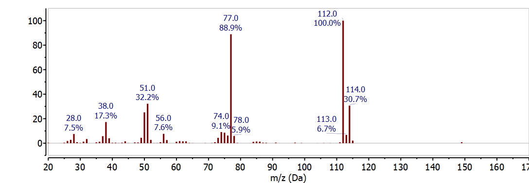
Chlorine Isotope Abundance

The natural abundance of these two isotopes is observed in the mass spectrum as two peaks separated by 2 m/z with a relative intensity of \(3: 1\). The mass spectrum of chlorobenzene C₆H₅Cl in Figure \(\PageIndex{1}\) clearly shows the chlorine isotope distribution at 112 m/z and 114 m/z . These peaks correspond to the molecular ion - the molecular ion has the most abundant isotope for each element - at 112 m/z (6x12 + 5x1 + 35) and the ³⁷Cl isotope peak at 114 m/z (6x12 + 5x1 + 37) and the relative intensity is determined by the natural abundance of the ³⁷Cl isotope. The other major peak in this spectrum at 77 m/z corresponds to the loss of chlorine from the molecular ion or the ³⁷Cl isotope peak to give C₆H₅⁺ (112 - 35 = 77 OR 114 - 37 = 77).

Figure \(\PageIndex{1}\): Mass Spectrum of chlorobenzene.

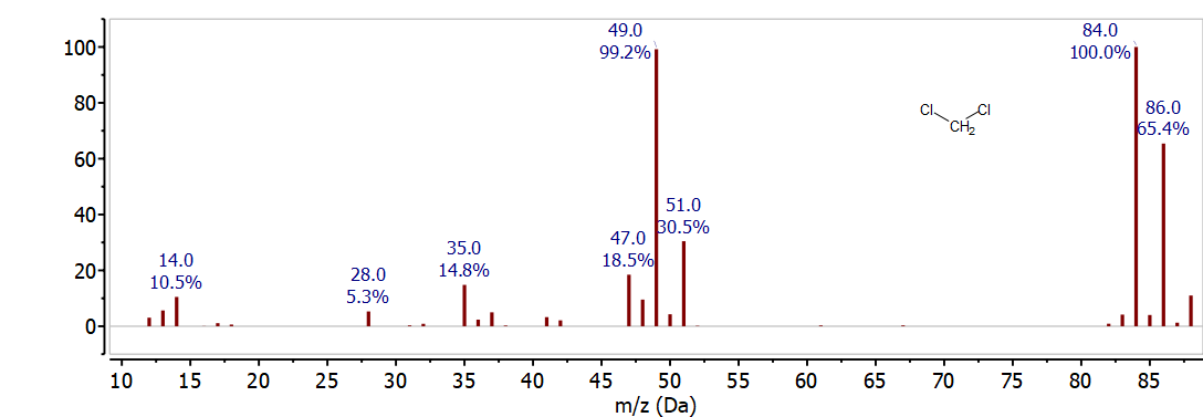
If more than one chlorine atom is present, the isotope abundance is more complex. An ion with two chlorine atoms has three possible isotope combinations. This pattern is apparent in the mass spectrum of CH₂Cl₂ shown in Figure \(\PageIndex{2}\). Ions are observed for \(\mathrm{CH}_{2}{ }^{35} \mathrm{Cl}_{2}^{+}\) at 84 m/z, \(\mathrm{CH}_{2}{ }^{35} \mathrm{Cl}^{37} \mathrm{Cl}^{+}\) at 86 m/z , and \(\mathrm{CH}_{2}{ }^{37} \mathrm{Cl}_{2}^{+}\) at 88 m/z . Based up on the probability of each combination of isotopes, the relative intensity of these peaks is \(10: 6: 1\). The \(3: 1\) isotope ratio for an ion with a single chlorine atom is observed at 49 m/z and 51 m/z . This corresponds to \(\mathrm{CH}_{2}{ }^{35} \mathrm{Cl}^{+}\)and \(\mathrm{CH}_{2}{ }^{37} \mathrm{Cl}^{+}\)fragments formed by loss of \(\mathrm{Cl}\) from the molecular ion. Careful examination of the spectrum also shows ions produced by loss of H^• and \(\mathrm{H}_{2}\).

Figure \(\PageIndex{2}\): Mass Spectrum of dichloromethane.

Bromine Isotope Abundance

Bromine also has two naturally occurring isotopes, ⁷⁹Br is the most abundant and ⁸¹Br has a relative abundance of 98% which results in a relative intensity for these two peaks of 1:1. This is observed in the mass spectrum of bromobenzene shown in Figure \(\PageIndex{3}\). The bromine isotope pattern is seen in the peaks at 156 m/z and 158 m/z which have the 1:1 relative abundance characteristic of bromine. These two peaks correspond to the molecular ion C₆H₅⁷⁹Br at 156 m/z and C₆H₅⁸¹Br at 158 m/z . The base peak in this spectrum is from loss of Br to form C₆H₅ observed at 77 m/z .

Figure \(\PageIndex{3}\): Mass Spectrum of bromobenzene.

Carbon 13 isotope peak

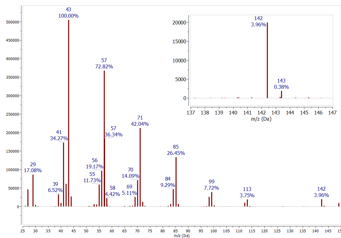
The \(1.1 \%\) of natural abundance of \({ }^{13} \mathrm{C}\) is another useful tool for interpreting mass spectra. The abundance of a peak one m/z value higher, where a single \({ }^{12} C\) is replaced by a \({ }^{13} C\), is determined by the number of carbons in the ion. The rule of thumb for small compounds is that each carbon atom in the ion increases the abundance of the \(M+1\) peak by \(1 \%\). This effect is seen in all the spectra discussed in this paper. For example, in the \(n\)-decane mass spectrum (Figure \(\PageIndex{4}\) ) compare the peak for \({ }^{12} \mathrm{C}_{9}{ }^{13} \mathrm{C}^{1} \mathrm{H}_{22}\) at 143 m/z (0.38 % relative abundance) to the peak for \({ }^{12} \mathrm{C}_{10}{ }^{1} \mathrm{H}_{22}\) at 142 m/z (3.96% relative abundance). The abundance of the \(13 \mathrm{C}\) peak is \(10 \%\) the abundance of the \({ }^{12} \mathrm{C}\) peak, consistent with a compound containing 10 carbon atoms. Now look at some previous spectra to find more examples of this pattern. Be aware that for compounds with low molecular ion abundances the uncertainty in measuring this ratio may be +/- several carbon atoms.

Figure \(\PageIndex{4}\): Mass Spectrum of Decane.

Isotope Abundances

Because all atoms have several naturally occurring isotopes, the patterns discussed here become more complex. Fortunately, most elements common in organic mass spectrometry have one predominant isotope. The high abundance of the two chlorine isotopes is unusual, so they are easy to identify. The relative abundances for isotopes of frequently encountered elements are given in Table \(\PageIndex{1}\). For molecules with more complex isotope patterns there are a number of programs and websites available for modeling the distributions. The calculator provided by Scientific Instrument Services is available at: https://www.sisweb.com/mstools/isotope.htm.

Table \(\PageIndex{1}\): Isotope Abundances. Adapted from McLafferty, F. Interpretation of Mass Spectra (University Science, Mill Valley CA: 1980.

Atom	Isotope A			Istope A+1			Isotope A+2
	mass	%		mass	%		mass	%
H	1	100		2	0.015
C	12	100		13	1.1
N	14	100		15	0.37
O	16	100		17	0.04		18	0.20
F	19	100
Si	28	100		29	5.1		30	3.4
P	31	100
S	32	100		33	0.80		34	4.4
Cl	35	100					37	32.5
Br	79	100					81	98.0
I	127	100